在 AMD GPU 上使用 JAX 实现和训练生成预训练变换器 (GPT) 的指南

2024年7月2日,由 Douglas Jia撰写。
在本文中,我们展示了如何在JAX中实现和训练生成预训练变换模型(GPT),参考了Andrej Karpathy基于PyTorch的 nanoGPT。通过对比在PyTorch和JAX中实现GPT模型的关键组件(如自注意力机制和优化器)的差异,我们阐明了JAX的独特属性。此外,我们还提供了GPT模型基础知识的入门概述,以增强理解。
背景
在数据科学和机器学习领域,框架的选择在模型开发和性能方面起着至关重要的作用。PyTorch 长期以来因为其直观的界面和动态计算图被研究人员和从业者所青睐。另一方面,JAX/Flax 提供了一种独特的方法,专注于函数式编程和可组合的函数变换。由谷歌开发的 JAX 提供了 Python 和 NumPy 代码的自动微分和可组合的函数变换。基于 JAX 构建的 Flax 提供了一个高级 API,用于定义和训练神经网络模型,同时利用 JAX 的自动微分和硬件加速能力。它旨在通过模块化的模型构建和对分布式训练的支持,提供灵活性和易用性。尽管 PyTorch 在灵活性方面表现出色,JAX 则在性能优化和硬件加速(特别是在 GPU 和 TPU 上)方面脱颖而出。此外,JAX 通过透明地在可用加速器上运行而无需明确的设备指定,简化了设备管理。
Andrej Karpathy 开发的 nanoGPT 是 GPT 语言模型的精简版本,这是一种在自然语言处理领域具有变革意义的深度学习架构。不同于 OpenAI 的资源密集型 GPT 模型,nanoGPT 被设计得轻量级,甚至可以在普通硬件设备上轻松部署。尽管其体积紧凑,nanoGPT 仍保留了 GPT 模型的核心功能,包括文本生成、语言理解及适应各种下游应用。它的重要性在于使尖端语言模型的访问更加民主化,使研究人员、开发者及爱好者即使在消费级 GPU 上也能深入探索自然语言 AI。
在这篇博客中,我们将带你走过将 PyTorch 定义的 GPT 模型和训练过程转换为 JAX/Flax 的过程,以 nanoGPT 为我们的指导示例。通过剖析在实现关键 GPT 模型组件和训练机制(如自注意力和优化器)方面的这些框架之间的差异,我们的目标是提供一份全面的比较指南,以掌握 JAX。此外,通过调整我们的 JAX nanoGPT 代码,我们为构建个性化 JAX 模型和训练框架提供了基础。这一努力提高了模型的灵活性和部署的便利性,促进了基于机器学习的 NLP 技术的广泛采纳和发展。在这篇博客的最后一部分,我们将展示如何使用字符级莎士比亚数据集预训练 nanoGPT-JAX 模型并生成样本输出。
如果你是一名熟悉 JAX/Flax 的经验丰富的开发人员,并且寻求能够帮助你的项目的实现细节,你可以直接访问我们所有源码在 rocm-blogs GitHub 页面。
将 PyTorch 模型定义和训练过程转换为 JAX
要训练和执行深度学习模型,包括大型语言模型(LLM),通常需要两个基本的文件:`model.py` 和 train.py。在 GPT 模型的上下文中,`model.py` 文件定义了架构,包含以下关键组件:
-
Token 和位置嵌入层;
-
多个块,每个块由一个注意力层和一个多层感知器(MLP)层组成,每个层之前都有一个归一化层,用于标准化沿序列维度的输入;
-
一个最终的线性层,通常被称为语言模型头,负责将 transformer 模型的输出映射到词汇分布。
train.py 文件则概述了训练过程。它包含以下重要组件:
-
数据加载器,负责在训练迭代期间按顺序提供随机采样的数据批次;
-
优化器,决定参数的更新;
-
训练状态,这是 Flax 特有的,负责管理和更新模型参数,以及其他组件如优化器和前向传播。需要注意的是,虽然 Flax 统一地将这些组件集成到一个训练状态中,PyTorch 则在训练循环中分别处理它们。
在本节中,我们将引导您逐步将 nanoGPT 模型和训练过程的关键组件从 PyTorch 转换为 JAX。为方便比较,我们将并排展示 PyTorch 和 JAX 代码模块。请注意,本节中的代码片段仅供说明用。它们不可执行,因为我们省略了执行所需但与主题无关的必要代码(例如,模块导入)。完整实现请参阅我们 GitHub 仓库中的 model.py 和 train.py 文件。
自注意力
GPT模型中的自注意力模块通过计算基于单词之间关系的注意力得分来衡量序列中单词的重要性。这使得有效捕捉长距离依赖关系和上下文信息成为可能,对于自然语言理解和生成等任务至关重要。
为了说明自注意力模块在PyTorch和JAX实现之间的差异,我们提供了对应的代码块。
| PyTorch | JAX/Flax |
|---|---|
class CausalSelfAttention(nn.Module):
    def __init__(self, config):
        super().__init__()
        assert config.n_embd % config.n_head == 0
        # 为所有头部计算键、查询和值投影,但在一个批次中
        self.c_attn = nn.Linear(config.n_embd, 3 * config.n_embd, bias=config.bias)
        # 输出投影
        self.c_proj = nn.Linear(config.n_embd, config.n_embd, bias=config.bias)
        # 正则化
        self.attn_dropout = nn.Dropout(config.dropout)
        self.resid_dropout = nn.Dropout(config.dropout)
        self.n_head = config.n_head
        self.n_embd = config.n_embd
        self.dropout = config.dropout
        # 闪存注意力使GPU运作更快,但仅支持PyTorch >= 2.0
        self.flash = hasattr(torch.nn.functional, "scaled_dot_product_attention")
        if not self.flash:
            print(
                "WARNING: using slow attention. Flash Attention \
                requires PyTorch >= 2.0"
            )
            # 因果掩码确保注意力仅应用于输入序列的左侧
            self.register_buffer(
                "bias",
                torch.tril(torch.ones(config.block_size, config.block_size)).view(
                    1, 1, config.block_size, config.block_size
                ),
            )

    def forward(self, x):
        # 批量大小、序列长度、嵌入维度(n_embd)
        (B, T, C,) = x.size()

        # 计算批次中所有头部的查询、键和值,并将头部前移以成为批次维度
        q, k, v = self.c_attn(x).split(self.n_embd, dim=2)
        k = k.view(B, T, self.n_head, C // self.n_head).transpose(
            1, 2
        )  # (B, nh, T, hs)
        q = q.view(B, T, self.n_head, C // self.n_head).transpose(
            1, 2
        )  # (B, nh, T, hs)
        v = v.view(B, T, self.n_head, C // self.n_head).transpose(
            1, 2
        )  # (B, nh, T, hs)

        # 因果自注意力;自我注意:(B, nh, T, hs) x
        # (B, nh, hs, T) -> (B, nh, T, T)
        if self.flash:
            # 使用Flash Attention CUDA内核进行高效注意力计算
            y = torch.nn.functional.scaled_dot_product_attention(
                q,
                k,
                v,
                attn_mask=None,
                dropout_p=self.dropout if self.training else 0,
                is_causal=True,
            )
        else:
            # 手动实现的注意力
            att = (q @ k.transpose(-2, -1)) * (1.0 / math.sqrt(k.size(-1)))
            att = att.masked_fill(self.bias[:, :, :T, :T] == 0, float("-inf"))
            att = F.softmax(att, dim=-1)
            att = self.attn_dropout(att)
            # (B, nh, T, T) x (B, nh, T, hs) -> (B, nh, T, hs)
            y = att @ v
        y = (
            y.transpose(1, 2).contiguous().view(B, T, C)
        )  # 将所有头部输出并列重新组合

        # 输出投影
        y = self.resid_dropout(self.c_proj(y))
        return y
| class CausalSelfAttention(nn.Module):
#GPTConfig 是一个定义模型架构的类,包括词汇表大小、块大小(上下文窗口长度)、注意力头的数量、嵌入维度等参数。详细信息请参见 model.py 文件中的 GPTConfig 类定义。
config: GPTConfig
@nn.compact
def __call__(self, x, train=False, rng1=None, rng2=None):
assert self.config.n_embd % self.config.n_head == 0
# 批量大小、序列长度、嵌入维度(n_embd)
(B, T, C,) = x.shape
# 计算批次中所有头部的查询、键和值,并将头部前移以成为批次维度
q, k, v = jnp.split(
nn.Dense(self.config.n_embd * 3, name="c_attn")(x), 3, axis=-1
)
k = k.reshape(B, T, self.config.n_head, C // self.config.n_head).swapaxes(
1, 2
) # (B, nh, T, hs)
q = q.reshape(B, T, self.config.n_head, C // self.config.n_head).swapaxes(
1, 2
) # (B, nh, T, hs)
v = v.reshape(B, T, self.config.n_head, C // self.config.n_head).swapaxes(
1, 2
) # (B, nh, T, hs)
att = (
jnp.einsum("bhts,bhqs->bhtq", q, k, optimize=True)
if self.config.use_einsum
else jnp.matmul(q, k.swapaxes(-2, -1))
) * (1.0 / jnp.sqrt(k.shape[-1]))
mask = jnp.tril(jnp.ones((T, T))).reshape((1, 1, T, T))
att = jnp.where(mask == 0, float("-inf"), att)
att = nn.softmax(att, axis=-1)
att = nn.Dropout(
self.config.dropout, name="attn_dropout", deterministic=not train
)(att, rng=rng1)
y = (
jnp.einsum("bhts,bhsq->bhtq", att, v, optimize=True)
if self.config.use_einsum
else jnp.matmul(att, v)
) # (B, nh, T, T) x (B, nh, T, hs) -> (B, nh, T, hs)
y = y.swapaxes(1, 2).reshape(
B, T, C
) # 重新组合所有头部输出并列
# 输出投影
y = nn.Dense(self.config.n_embd, name="c_proj")(y)
y = nn.Dropout(
self.config.dropout, name="resid_dropout", deterministic=not train
)(y, rng=rng2)
return y
|
在上面的并排比较中,你会注意到在`CausalSelfAttention`类中,PyTorch需要一个`__init__方法来初始化所有层,一个forward`方法来定义计算过程,通常称为“前向传递”。相比之下,Flax提供了一种更简洁的方法:你可以利用使用`@nn.compact`装饰的`__call__`方法来内联初始化层并同时定义计算过程。这导致JAX/Flax的实现明显比PyTorch短和简洁。
为了方便从PyTorch迁移到JAX/Flax,Flax引入了`setup`方法,它相当于`__init__。使用setup`方法,你可以初始化所有层,并使用`__call__方法(无需@nn.compact`装饰器)来执行前向传递。当定义GPT类时,将演示这种方法。请注意,与`setup`方法相比,`nn.compact`的行为并无不同;这只是个人习惯问题。
另一个显著的区别是,尽管PyTorch要求为层指定输入和输出形状,Flax只需指定输出形状,因为它可以根据提供的输入推断出输入形状。这一特性在输入形状未知或初始化时难以确定时尤为有用。
定义GPT模型
一旦定义了`CausalSelfAttention`类,我们接下来将定义`MLP`类,并将这两个类组合成一个`Block`类。随后,在主要的`GPT`类中,我们将整合这些元素——嵌入层、包含注意力和MLP层的块以及语言模型头——构建GPT模型。值得注意的是,`Block`层结构将在GPT模型中重复`n_layer`次。这种重复有助于分层特征学习,使模型能够在不同抽象级别捕捉输入数据的各个方面,并逐步捕捉更复杂的模式和依赖关系。
| PyTorch | JAX/Flax |
|---|---|
class MLP(nn.Module):
    def __init__(self, config):
        super().__init__()
        self.c_fc = nn.Linear(config.n_embd, 4 * config.n_embd, bias=config.bias)
        self.gelu = nn.GELU()
        self.c_proj = nn.Linear(4 * config.n_embd, config.n_embd, bias=config.bias)
        self.dropout = nn.Dropout(config.dropout)

    def forward(self, x):
        x = self.c_fc(x)
        x = self.gelu(x)
        x = self.c_proj(x)
        x = self.dropout(x)
        return x


class Block(nn.Module):
    def __init__(self, config):
        super().__init__()
        self.ln_1 = LayerNorm(config.n_embd, bias=config.bias)
        self.attn = CausalSelfAttention(config)
        self.ln_2 = LayerNorm(config.n_embd, bias=config.bias)
        self.mlp = MLP(config)

    def forward(self, x):
        x = x + self.attn(self.ln_1(x))
        x = x + self.mlp(self.ln_2(x))
        return x


class GPT(nn.Module):
    def __init__(self, config):
        super().__init__()
        assert config.vocab_size is not None
        assert config.block_size is not None
        self.config = config

        self.transformer = nn.ModuleDict(
            dict(
                wte=nn.Embedding(config.vocab_size, config.n_embd),
                wpe=nn.Embedding(config.block_size, config.n_embd),
                drop=nn.Dropout(config.dropout),
                h=nn.ModuleList([Block(config) for _ in range(config.n_layer)]),
                ln_f=LayerNorm(config.n_embd, bias=config.bias),
            )
        )
        self.lm_head = nn.Linear(config.n_embd, config.vocab_size, bias=False)
        self.transformer.wte.weight = self.lm_head.weight

        # 初始化所有权重
        self.apply(self._init_weights)
        # 对残差投影进行特殊的比例初始化,参考GPT-2论文
        for pn, p in self.named_parameters():
            if pn.endswith("c_proj.weight"):
                torch.nn.init.normal_(
                    p, mean=0.0, std=0.02 / math.sqrt(2 * config.n_layer)
                )

        # 报告参数数量
        print("number of parameters: %.2fM" % (self.get_num_params() / 1e6,))

    def forward(self, idx, targets=None):
        device = idx.device
        b, t = idx.size()
        assert (
            t <= self.config.block_size
        ), f"Cannot forward sequence of length {t}, block size is only {
            self.config.block_size}"
        pos = torch.arange(0, t, dtype=torch.long, device=device)  # shape (t)

        # 前向传递GPT模型本身
        tok_emb = self.transformer.wte(idx)  # token embd shape (b, t, n_embd)
        pos_emb = self.transformer.wpe(pos)  # position embd shape (t, n_embd)
        x = self.transformer.drop(tok_emb + pos_emb)
        for block in self.transformer.h:
            x = block(x)
        x = self.transformer.ln_f(x)

        if targets is not None:
            # 如果给定了一些目标同时计算损失
            logits = self.lm_head(x)
            loss = F.cross_entropy(
                logits.view(-1, logits.size(-1)), targets.view(-1), ignore_index=-1
            )
        else:
            # 推理时间的小优化:仅对最后一个位置前向传递lm_head
            # very last position
            logits = self.lm_head(
                x[:, [-1], :]
            )  # 注意:使用列表[-1]以保留时间维度
            loss = None

        return logits, loss
| class MLP(nn.Module):
config: GPTConfig
@nn.compact
def __call__(self, x, train=False, rng=None):
x = nn.Dense(4 * self.config.n_embd, use_bias=self.config.bias)(x)
x = nn.gelu(x)
x = nn.Dense(self.config.n_embd, use_bias=self.config.bias)(x)
x = nn.Dropout(self.config.dropout, deterministic=not train)(x, rng=rng)
return x
class Block(nn.Module):
config: GPTConfig
@nn.compact
def __call__(self, x, train=False, rng1=None, rng2=None, rng3=None):
x = x + CausalSelfAttention(self.config, name="attn")(
nn.LayerNorm(use_bias=self.config.bias, name="ln_1")(x),
train=train,
rng1=rng1,
rng2=rng2,
)
x = x + MLP(self.config, name="mlp")(
nn.LayerNorm(use_bias=self.config.bias, name="ln_2")(x),
train=train,
rng=rng3,
)
return x
class GPT(nn.Module):
config: GPTConfig
def setup(self):
assert self.config.vocab_size is not None
assert self.config.block_size is not None
self.wte = nn.Embed(self.config.vocab_size, self.config.n_embd)
self.wpe = nn.Embed(self.config.block_size, self.config.n_embd)
self.drop = nn.Dropout(self.config.dropout)
self.h = [Block(self.config) for _ in range(self.config.n_layer)]
self.ln_f = nn.LayerNorm(use_bias=self.config.bias)
def __call__(self, idx, targets=None, train=False, rng=jax.random.key(0)):
_, t = idx.shape
assert (
t <= self.config.block_size
), f"Cannot forward sequence of length {t}, block size is only {
self.config.block_size}"
pos = jnp.arange(t, dtype=jnp.int32)
# forward the GPT model itself
tok_emb = self.wte(idx) # token embeddings of shape (b, t, n_embd)
pos_emb = self.wpe(pos) # position embeddings of shape (t, n_embd)
rng0, rng1, rng2, rng3 = jax.random.split(rng, 4)
x = self.drop(tok_emb + pos_emb, deterministic=False, rng=rng0)
for block in self.h:
x = block(x, train=train, rng1=rng1, rng2=rng2, rng3=rng3)
x = self.ln_f(x)
if targets is not None:
# weight tying (https://github.com/google/flax/discussions/2186)
logits = self.wte.attend(
x
) # (b, t, vocab_size)
loss = optax.softmax_cross_entropy_with_integer_labels(
logits, targets
).mean()
else:
logits = self.wte.attend(x[:, -1:, :])
loss = None
return logits, loss
|
在上面的JAX/Flax实现中,您会注意到我们使用了`@nn.compact`装饰器将初始化和前向传递整合在了`__call__方法中,对于MLP`和`Block`类均是如此。然而,在`GPT`类中,我们选择了使用`setup`方法来进行初始化,`__call__方法进行前向传递。这一点与PyTorch和Flax的差异之一就在于权重共享的指定,这涉及到在嵌入层和输出层(语言模型头部)之间共享权重。权重共享非常有益,因为这两者的矩阵通常捕捉到相似的语义属性。在PyTorch中,权重共享通过self.transformer.wte.weight = self.lm_head.weight`来完成,而在Flax中是通过`self.wte.attend`方法实现的。此外,在JAX中,当涉及到引入随机性时,需要明确指定一个随机数生成器密钥,而在PyTorch中则不需要这一步。
优化器
优化器在训练深度学习模型中起到关键作用,通过定义更新规则和策略来调整模型参数。它们还可以整合诸如权重衰减之类的正则化技术,以防止过拟合并增强泛化能力。
一些流行的优化器包括:
-
带动量的随机梯度下降 (SGD) with Momentum: 这种优化器引入了动量项,以加速在最近梯度方向上的参数更新。
-
Adam: Adam结合了动量和均方根传播(RMSprop)的优点,基于梯度和平方梯度的移动平均值,为每个参数动态调整学习率。
-
AdamW: Adam的一种变体,包含了权重衰减,通常用于各种深度学习任务。
在训练大型语言模型(LLMs)时,通常选择性地对参与矩阵乘法 (详见安德烈·卡普西蒂的评论)的层应用权重衰减。
在下面的代码示例中,观察PyTorch和JAX由于使用的数据结构不同,在处理权重衰减上的差异。想要深入了解的读者可以探索 这个关于PyTrees的教程。
| PyTorch | JAX/Flax |
|---|---|
def configure_optimizers(self, weight_decay, learning_rate, betas, device_type):
    # 从所有候选参数开始
    param_dict = {pn: p for pn, p in self.named_parameters()}
    # 过滤掉那些不需要梯度的参数
    param_dict = {pn: p for pn, p in param_dict.items() if p.requires_grad}
    # 创建优化组。任何2D的参数将会被应用权重衰减,
    # 其他的则不会。即所有在矩阵乘法和嵌入中的权重张量衰减,
    # 所有偏置和层归一化则不衰减。
    decay_params = [p for n, p in param_dict.items() if p.dim() >= 2]
    nodecay_params = [p for n, p in param_dict.items() if p.dim() < 2]
    optim_groups = [
        {"params": decay_params, "weight_decay": weight_decay},
        {"params": nodecay_params, "weight_decay": 0.0},
    ]
    # 创建AdamW优化器,并在如果可用的情况下,使用融合版本
    fused_available = "fused" in inspect.signature(torch.optim.AdamW).parameters
    use_fused = fused_available and device_type == "cuda"
    extra_args = dict(fused=True) if use_fused else dict()
    optimizer = torch.optim.AdamW(
        optim_groups, lr=learning_rate, betas=betas, **extra_args
    )
    print(f"using fused AdamW: {use_fused}")

    return optimizer
| def configure_optimizers(self, params, weight_decay, learning_rate, betas):
# 仅对涉及矩阵乘法的权重实现权重衰减。
label_fn = (
lambda path, value: "no_decay"
if (value.ndim < 2) or ("embedding" in path)
else "decay"
)
# 创建优化组
decay_opt = optax.adamw(
learning_rate, weight_decay=weight_decay, b1=betas[0], b2=betas[1]
)
nodecay_opt = optax.adam(learning_rate, b1=betas[0], b2=betas[1])
tx = optax.multi_transform(
{"decay": decay_opt, "no_decay": nodecay_opt},
flax.traverse_util.path_aware_map(label_fn, params),
)
return tx
|
训练循环
训练循环涉及在数据集上迭代训练模型的过程,包括以下步骤:
-
数据加载: 使用数据加载函数从数据集中批量加载训练数据,通常是文本序列。
-
前向传播: 将输入序列通过模型传播以生成预测结果。
-
损失计算: 确定模型预测与实际目标(例如序列中的下一个单词)之间的损失。
-
反向传播(梯度计算): 通过反向传播计算损失相对于模型参数的梯度。
-
参数更新: 使用优化器基于计算出的梯度调整模型参数。
-
重复上述步骤: 重复步骤2到步骤5。
训练循环旨在最小化损失函数并优化模型参数,以便在未见过的数据上进行准确预测。 在本节中,我们仅展示JAX/Flax的实现,使用一个统一的训练状态类来存储模型、参数和优化器,执行诸如前向传播和参数更新等基本步骤。JAX的方法与PyTorch的设计有显著不同,因此直接进行并排比较可能并不有利。感兴趣的读者可以自行进行比较,参考PyTorch实现。
训练状态
在下面的代码块中,你会注意到变量 state 的 train_state 类包含了模型的前向传递定义、优化器和参数。Flax 与 PyTorch 不同的地方在于,它将模型和参数分离为两个变量。要初始化参数,必须提供一些示例数据给定义好的模型,以便通过这些数据推断层的形状。因此,可以将 model 看作是定义前向传递架构的固定变量,而在训练循环中更新的是 state 持有的其他变量,例如参数和优化器。
# 定义初始化训练状态的函数
def init_train_state(
    model,
    params,
    learning_rate,
    weight_decay=None,
    beta1=None,
    beta2=None,
    decay_lr=True,
    warmup_iters=None,
    lr_decay_iters=None,
    min_lr=None,
) -> train_state.TrainState:
    # 学习率衰减调度器(使用热身的余弦衰减)
    if decay_lr:
        assert warmup_iters is not None, "warmup_iters must be provided"
        assert lr_decay_iters is not None, "lr_decay_iters must be provided"
        assert min_lr is not None, "min_lr must be provided"
        assert (
            lr_decay_iters >= warmup_iters
        ), "lr_decay_iters must be greater than or equal to warmup_iters"
        lr_schedule = optax.warmup_cosine_decay_schedule(
            init_value=1e-9,
            peak_value=learning_rate,
            warmup_steps=warmup_iters,
            decay_steps=lr_decay_iters,
            end_value=min_lr,
        )
    else:
        lr_schedule = learning_rate
    # 创建优化器
    naive_optimizer = model.configure_optimizers(
        params,
        weight_decay=weight_decay,
        learning_rate=lr_schedule,
        betas=(beta1, beta2),
    )
    # 添加梯度裁剪
    optimizer = optax.chain(optax.clip_by_global_norm(grad_clip), naive_optimizer)
    # Create a State
    return (
        train_state.TrainState.create(
            apply_fn=model.apply, tx=optimizer, params=params
        ),
        lr_schedule,
    )


model = GPT(gptconf)
# idx 是用于初始化参数的虚拟输入
idx = jnp.ones((3, gptconf.block_size), dtype=jnp.int32)
params = model.init(jax.random.PRNGKey(1), idx)
state, lr_schedule = init_train_state(
    model,
    params["params"],
    learning_rate,
    weight_decay,
    beta1,
    beta2,
    decay_lr,
    warmup_iters,
    lr_decay_iters,
    min_lr,
)
训练步骤
train_step 函数组织了反向传播过程,该过程基于前向传播的损失计算梯度,并随后更新 state 变量。它接受 state 作为参数并返回更新后的 state,整合来自当前数据批次的信息。值得注意的是,我们显式地提供了一个随机数键 rng 给 train_step 函数,以确保 dropout 层的正常运行。
def loss_fn(params, x, targets=None, train=True, rng=jax.random.key(0)):
    _, loss = state.apply_fn(
        {"params": params}, x, targets=targets, train=train, rng=rng
    )
    return loss

# 以下函数对 `train_step` 函数进行 JIT 编译。`jax.value_and_grad(loss_fn)` 创建一个能够同时评估 `loss_fn` 及其梯度的函数。作为常见做法,你只需对最外层的函数进行 JIT 编译。
@partial(jax.jit, donate_argnums=(0,))
def train_step(
    state: train_state.TrainState,
    batch: jnp.ndarray,
    rng: jnp.ndarray = jax.random.key(0),
):
    x, y = batch
    key0, key1 = jax.random.split(rng)
    gradient_fn = jax.value_and_grad(loss_fn)
    loss, grads = gradient_fn(state.params, x, targets=y, rng=key0, train=True)
    state = state.apply_gradients(grads=grads)
    return state, loss, key1
循环
这是训练过程的最后一步:定义训练循环。在这个循环中,`train_step` 函数将通过每个数据批次迭代更新 state。循环将持续进行,直到满足终止条件,比如超出预设的最大训练迭代次数。
while True:

    if iter_num == 0 and eval_only:
        break

    state, loss, rng_key = train_step(state, get_batch("train"), rng_key)

    # 计时和记录
    t1 = time.time()
    dt = t1 - t0
    t0 = t1
    iter_num += 1

    # 终止条件
    if iter_num > max_iters:
        break
请注意,实际的训练循环比上面展示的要复杂,因为它通常包括评估和检查点步骤以及其他记录步骤,这些步骤有助于监控训练进度和调试。保存的检查点可用于恢复训练或后续推理。然而,由于篇幅限制,我们忽略了这些部分。感兴趣的读者可以深入研究我们的源代码以进行进一步探索。
实现步骤
接下来,我们将引导您设置运行环境、启动训练和微调,并使用最终训练好的检查点生成文本。
环境设置
我们在一个运行PyTorch ROCm 6.1的Docker容器 (check the list of supported OSs and AMD hardware) 中使用AMD GPU进行了实现,以便在PyTorch和JAX之间进行比较,因为原始的nanoGPT是用PyTorch实现的。我们将在容器中安装包括JAX和Jaxlib在内的必要软件包。请注意,尽管我们在博客中使用了AMD GPU,但我们的代码没有包含任何特定于AMD的修改。这突显了ROCm对主要深度学习框架如PyTorch和JAX的适应性。
首先,在Linux Shell中通过如下代码拉取并运行Docker容器:
docker run -it --ipc=host --network=host --device=/dev/kfd --device=/dev/dri \
           --group-add video --cap-add=SYS_PTRACE --security-opt seccomp=unconfined \
           --name=nanogpt rocm/pytorch:rocm6.1_ubuntu22.04_py3.10_pytorch_2.1.2 /bin/bash
接下来,在Docker容器中执行以下代码,以安装必要的Python软件包并配置XLA的环境变量:
python3 -m pip install --upgrade pip
pip install optax==0.2.2 flax==0.8.2 transformers==4.38.2 tiktoken==0.6.0 datasets==2.17.1
python3 -m pip install https://github.com/ROCmSoftwarePlatform/jax/releases/download/jaxlib-v0.4.26/jaxlib-0.4.26+rocm610-cp310-cp310-manylinux2014_x86_64.whl
python3 -m pip install https://github.com/ROCmSoftwarePlatform/jax/archive/refs/tags/jaxlib-v0.4.26.tar.gz
pip install numpy==1.22.0
export XLA_FLAGS="--xla_gpu_autotune_level=0"
然后,通过以下命令从 ROCm/rocm-blogs GitHub 仓库下载用于本博客的文件:
git clone https://github.com/ROCm/rocm-blogs.git
cd rocm-blogs/blogs/artificial-intelligence/nanoGPT-JAX
确保后续的所有操作都在 nanoGPT-JAX 文件夹内进行。
预训练一个 nanoGPT 模型
nanoGPT 原始仓库 提供了训练 GPT 模型的多种数据集处理管道。例如,您可以使用字符级莎士比亚数据集来训练 nanoGPT 模型,或使用莎士比亚或 OpenWebText 数据集来训练 GPT2 模型(或其他 GPT2 模型变体,如 GPT2-medium)。在本节中,我们将演示如何实现预训练和微调。您可以自定义数据集处理管道和配置文件,以使用其他数据集预训练或微调您感兴趣的模型。
# 预处理字符级莎士比亚数据集
python data/shakespeare_char/prepare.py
# 开始预训练
# 提供的配置文件设置了使用 JAX 在 AMD GPU 上训练一个微型字符级 GPT 模型。它指定了模型架构参数、训练设置、评估间隔、日志偏好、数据处理和检查点详细信息,确保了一个全面但灵活的实验和调试模型的设置。
python train.py config/train_shakespeare_char.py
预训练开始后,您会看到类似于以下的输出。注意,在前几十次迭代中,损失迅速减少。
Evaluating at iter_num == 0...
step 0: train loss 4.3827, val loss 4.3902; best val loss to now: 4.3902
iter 0: loss 4.4377, time 41624.53ms
iter 10: loss 3.4575, time 92.16ms
iter 20: loss 3.2899, time 88.92ms
iter 30: loss 3.0639, time 84.89ms
iter 40: loss 2.8163, time 85.28ms
iter 50: loss 2.6761, time 86.26ms
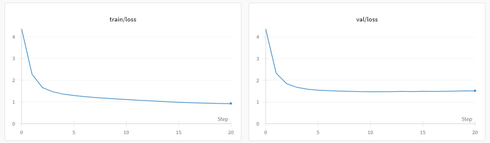
第一个步骤(iter 0)耗时明显比后续步骤更长。这是因为在第一次步骤中,JAX 编译模型和训练循环以优化计算,从而在未来的迭代中实现更快的执行速度。根据您使用的硬件,预训练过程可能需要几分钟到几十分钟的时间才能完成。您会注意到,通常在 2000 到 3000 次迭代之间会实现最佳验证损失。在达到最佳验证损失后,训练损失可能会继续减少,但验证损失可能会开始增加。这种现象被称为过拟合。我们在上图中展示了一个训练和验证损失的示例图。
Fine-tune GPT2-medium 模型
您还可以微调 GPT2 模型,以利用预训练模型的权重生成莎士比亚风格的文本。这意味着我们将使用相同的莎士比亚数据集,但使用 GPT2 模型架构而不是 nanoGPT 架构。在下面的示例中,我们微调了 gpt2-medium 模型。
# 预处理莎士比亚数据集
python data/shakespeare/prepare.py
# 开始微调
python train.py config/finetune_shakespeare.py
在初始迭代中,生成的输出将类似于以下内容:
Evaluting at iter_num == 0...
step 0: train loss 3.6978, val loss 3.5344; best val loss to now: 3.5344
iter 0: loss 4.8762, time 74683.51ms
iter 5: loss 4.9065, time 211.08ms
iter 10: loss 4.4118, time 250.01ms
iter 15: loss 4.9343, time 238.35ms
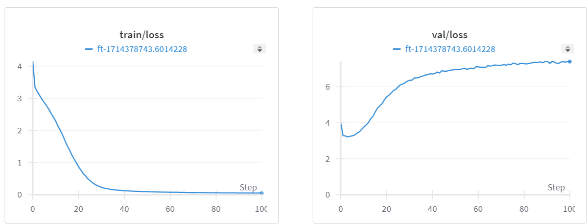
下图的损失曲线清楚地表明在验证数据上过拟合。
从保存的检查点生成样本
现在我们已经获得了预训练的字符级 nanoGPT 模型和微调的 GPT2-medium 模型的检查点,我们可以继续从这些检查点生成一些样本。我们将使用 sample.py 文件,以“\n”(新行)作为提示符生成三个样本。同时也可以尝试其他提示符。
# 从字符级 nanoGPT 模型生成样本
python sample.py --out_dir=out-shakespeare-char
你将会看到如下的输出:
Overriding: out_dir = out-shakespeare-char
Loading meta from data/shakespeare_char/meta.pkl...

Generated output __0__:
__________________________________

MBRCKaGEMESCRaI:Conuple to die with him.

MERCUTIO:
There's no sentence of him with a more than a right!

MENENIUS:
Ay, sir.

MENENIUS:
I have forgot you to see you.

MENENIUS:
I will keep you how to say how you here, and I say you all.

BENVOLIO:
Here comes you this last.

MERCUTIO:
That will not said the princely prepare in this; but you
will be put to my was to my true; and will think the
true cannot come to this weal of some secret but your conjured: I think
the people of your countrying hat
__________________________________

Generated output __1__:
__________________________________

BRCAMPSMNLES:
GREGod rathready and throng fools.

ANGELBOLINA:
And then shall not be more than a right!

First Murderer:
No, nor I: if my heart it, my fellows of our common
prison of Servingman:
I think he shall not have been my high to visit or wit.

LEONTES:
It is all the good to part it of my fault:
And this is mine, one but not that I was it.

First Lord:
But 'tis better knowledge, and merely away
good Capulet: were your honour to be here at all the good
And the banished of your country'st s
__________________________________

Generated output __2__:
__________________________________

SLCCESTEPSErShCnardareRoman:
Nay?

The garden hath aboard to see a fellow. Will you more than warrant!

First Murderer:
No, nor I: if my heart it, my fellows of your time is,
and you joy you how to save your rest life, I know not her;
My lord, I will be consul to Ireland
To give you and be too possible.

Second Murderer:
Ay, the gods the pride peace of Lancaster and Montague.

LADY GREY:
God give him, my lord; my lord.

KING EDWARD IV:
Poor cousin, intercept of the banishment.

HASTINGS:
The tim
__________________________________
现在,让我们使用微调的 GPT2-medium 模型生成样本:
# 从微调的 GPT2-medium 模型生成样本
python sample.py --out_dir=out-shakespeare --max_new_tokens=60
你将会看到如下的输出:
Overriding: out_dir = out-shakespeare
Overriding: max_new_tokens = 60
No meta.pkl found, assuming GPT-2 encodings...

Generated output __0__:
__________________________________


PERDITA:
It took me long to live, to die again, to see't.

DUKE VINCENTIO:
Why, then, that my life is not so dear as it used to be
And what I must do with it now, I know
__________________________________

Generated output __1__:
__________________________________


RICHARD:
Farewell, Balthasar, my brother, my friend.

BALTHASAR:
My lord!

VIRGILIA:
BALTHASAR,
As fortune please,
You have been a true friend to me.
__________________________________

Generated output __2__:
__________________________________


JULIET:
O, live, in sweet joy, in the sight of God,
Adonis, a noble man's son,
In all that my queen is,
An immortal king,
As well temperate as temperate!

All:
O Juno
__________________________________
通过对比这两个检查点生成的输出,我们可以观察到字符级的 nanoGPT 模型生成的文本尽管具备莎士比亚风格,但通常显得意义不明,而微调后的模型生成的文本可读性更强,证明了通过特定任务的数据集微调自定义大型语言模型以满足特定使用场景的有效性。
尽管这个教程到此结束,但我们希望它能够成为你探索、理解、编写代码和在不同框架(如 PyTorch 和 JAX/Flax)中实验大型语言模型的起点。
致谢和许可
我们衷心感谢Andrej Karpathy开发的基于PyTorch实现的nanoGPT代码库, 为我们的工作奠定了基础。没有他杰出的贡献,我们的项目将无法实现。在我们当前的工作中,我们重新编写了原始nanoGPT代码库中的三个文件:`model.py`、`sample.py`和`train.py`。
此外,我们还要感谢Cristian Garcia的nanoGPT-jax代码库, 它为我们的工作提供了宝贵的参考。

北京人形旗下天工造物具身智能开源社区,聚焦具身天工与慧思开物两大平台
更多推荐
 46
46 0
0- 0


 已为社区贡献4条内容

所有评论(0)