时序分析 34

时序预测 从ARIMA到SARIMAX(三) Box-Jenkins方法

上一篇我们进行了数据探索，本篇我们将介绍Box-Jenkins时序预测方法论，并开始进行ARIMA建模。

Step 3. Box-Jenkins Method 方法简介

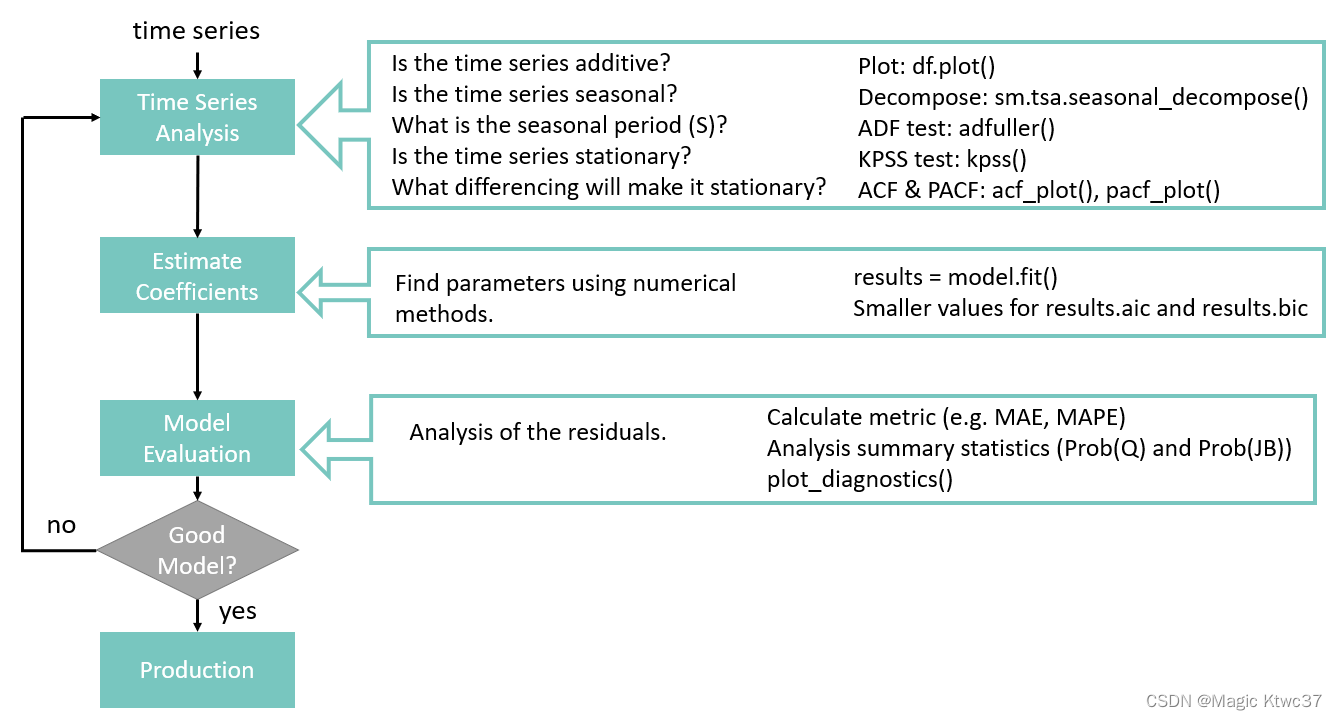
为了实践整个(S)ARIMA(X)模型构建过程，我们将参考Box-Jenkins Method。请参考下图，

此数据集种有500个时序，我们只针对2号仓库的28号商品进行预测建模。
我们将尝试回答如下问题：

• 时序是否平稳
• 如果时序不平稳，如何将其转换成平稳。
• 时序是否有季节性
• 如果具备季节性，那么周期是多长时间？
• 时序的各个组成成分的阶数是多少？（AR的p,MA的q)

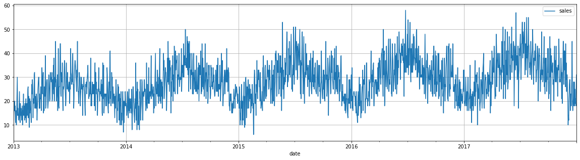
对仓库2的第28号商品进行可视化

df_store_2_item_28 = df_store_2[['date','sales']][df_store_2['item']==1].reset_index(drop=True)
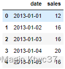
df_store_2_item_28.head()

# set date as index 
df_store_2_item_28_time = df_store_2_item_28.set_index('date')

# Plot the entire time series diet and show gridlines
df_store_2_item_28_time.plot(grid=True,figsize=(20,5))
plt.show()

from pylab import rcParams
rcParams['figure.figsize'] = 11, 9

import statsmodels.api as sm

decomposition = sm.tsa.seasonal_decompose(df_store_2_item_28_time, 
                                          model = 'additive',
                                          period=365, # cycle repeats 365 days, i.e., every year
                                         ) 
fig = decomposition.plot()
plt.show()

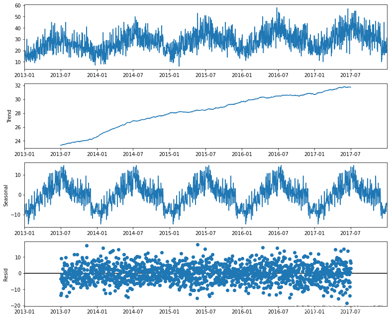
从上面的时序分解图中，我们可以得出如下结论：

• 1. 销售量有增长的趋势，因此时序数据是非平稳的。
• 2. 从季节性成分来看，季节模型应该是加性的，因为季节规律是稳定的。
• 3. 一月销售量最低，七月销售量最高。

进行平稳性检测

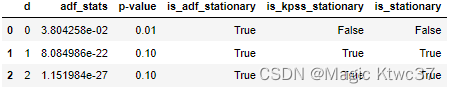
obtain_adf_kpss_results(df_store_2_item_28_time,3)

$d=1$就可以了。

画出ACF和PACF

在时序分析中，ACF和PACF图是常用分析工具。它们可以帮助我们发现时序的特性并协助估测ARIMA模型的参数。

from statsmodels.graphics.tsaplots import plot_acf, plot_pacf

# Create figure
fig, (ax1, ax2) = plt.subplots(2,1, figsize=(12,8))
 
# Plot the ACF of df_store_2_item_28_timeon ax1
plot_acf(df_store_2_item_28_time,lags=14, zero=False, ax=ax1)

# Plot the PACF of df_store_2_item_28_timeon ax2
plot_pacf(df_store_2_item_28_time,lags=14, zero=False, ax=ax2)

plt.show()

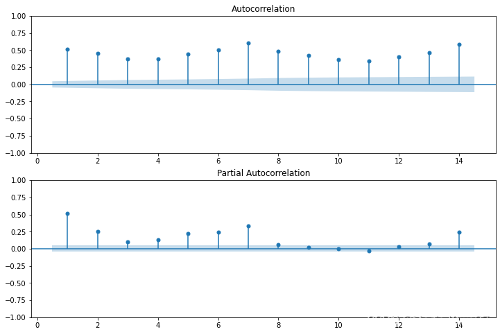
上面的图中，我们可以看到峰值出现在7和14，这说明季节成分7天（一周)重复一次。
下面画出一阶差分后的时序的ACF和PACF。

# Create figure
fig, (ax1, ax2) = plt.subplots(2,1, figsize=(12,8))
 
# Plot the ACF of df_store_2_item_28_timeon ax1
plot_acf(df_store_2_item_28_time.diff().dropna(),lags=14, zero=False, ax=ax1)

# Plot the PACF of df_store_2_item_28_timeon ax2
plot_pacf(df_store_2_item_28_time.diff().dropna(),lags=14, zero=False, ax=ax2)

plt.show()

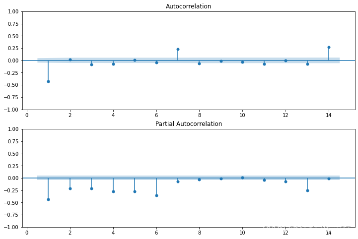
上面的图中并没有给我们带来多少新信息，同样只开到了季节性因素(周期为7)，这说明SARIMA模型可能会更为合适。

Step 4. 估算参数(p,q)

虽然我们知道SARIMA模型更适合于这个时序数据，我们还是从ARIMA模型开始。虽然ACF和PACF告诉了我们关于模型参数的不少信息，但我们还是应该依靠AIC (Akaike information criterion)和BIC (Bayesian information criterion)。

df_store_2_item_28_time.index = pd.DatetimeIndex(df_store_2_item_28_time.index.values,
                               freq=df_store_2_item_28_time.index.inferred_freq)

from statsmodels.tsa.statespace.sarimax import SARIMAX

# just an example
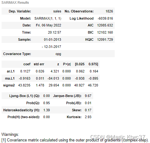
model = SARIMAX(df_store_2_item_28_time, order=(1,1,1), freq='D')
results = model.fit()
# statistics of the model
results.summary()

下面我们尝试不同的模型参数。

# Create empty list to store search results
order_aic_bic=[]

# Loop over p values from 0-6
for p in range(7):
  # Loop over q values from 0-6
    for q in range(7):
      	# create and fit ARMA(p,q) model
        model = SARIMAX(df_store_2_item_28_time, order=(p,1,q), freq="D") #because adf test showed that d=1
        results = model.fit()
        
        # Append order and results tuple
        order_aic_bic.append((p,q,results.aic, results.bic))

# Construct DataFrame from order_aic_bic
order_df = pd.DataFrame(order_aic_bic, 
                        columns=['p','q','AIC','BIC'])

# Print order_df in order of increasing AIC
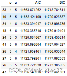
order_df.sort_values('AIC').head(10)

order_df.sort_values('BIC').head(10)

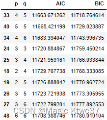
从AIC和BIC准则中，ARIMA(4,1,5)是最好的选择。

Step 5. 模型评价

在应用一个模型之前，我们希望能够了解模型的准确度。下面介绍了一些方法来评价一个模型。

MAE(Mean Absolute Error)

我们先计算一下残差的MAE

arima_model = SARIMAX(df_store_2_item_28_time, order=(4,1,5))
# fit model
arima_results = arima_model.fit()

# Calculate the mean absolute error from residuals
mae = np.mean(np.abs(arima_results.resid))

# Print mean absolute error
print('MAE: %.3f' % mae)

MAE: 4.729

df_store_2_item_28_time.describe()

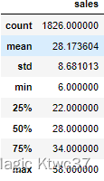
MAE接近5，而销量平均值为28.
一个好的模型应该使残差是非相关的高斯白噪声，且均值趋于0.下面我们来检查这一点。

摘要统计诊断

arima_results.summary()

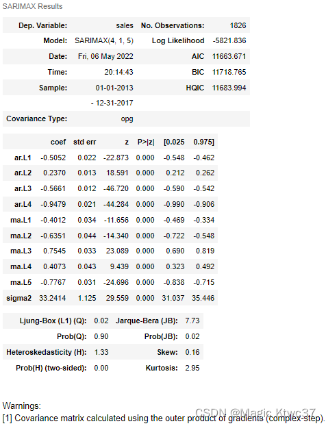
• Liung-box检验（原假设：残差不相关)，Prob(Q)=0.9 > 0.05，说明我们不能拒绝原假设，所以我们认为残差是不相关的。
• Jarque-Beta检验(原假设：残差为正态分布）,Prob(JB)=0.02 < 0.05，说明我们可以拒绝原假设，所以我们认为残差不是正态分布。

画出诊断图

# Create the 4 diagostics plots using plot_diagnostics method
arima_results.plot_diagnostics()
plt.show()

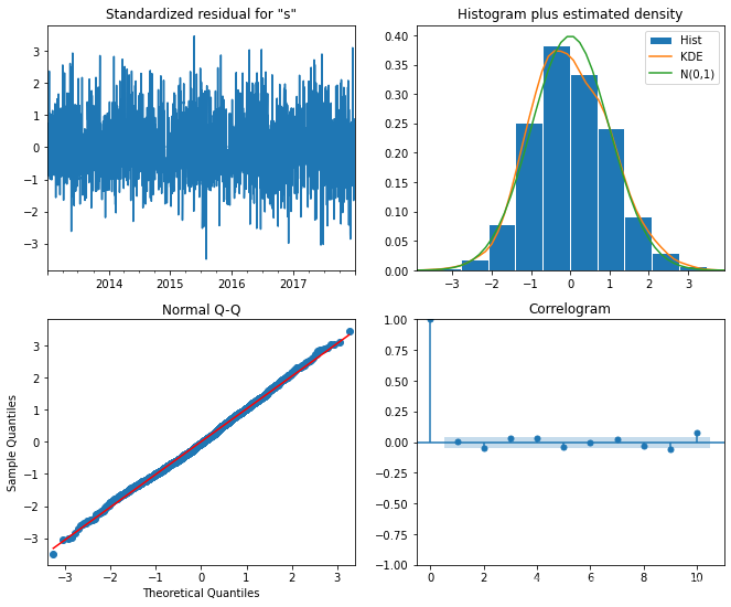
• Standardlized residul：残差并不存在明显的模式，这说明模型不错。
• Histogram plus KDE：残差的KDE曲线与标准正态分布的曲线存在一定的差距。
• Correlogram（ACF)：自相关都比较小，说明模型效果不错。
• Normal Q-Q：接近直线，说明残差是近似正态分布的，模型效果不错。
  整体看来，ARIMA模型的效果还是非常不错的。

小技巧：

如果残差与正态分布相距较远，可以尝试增加差分阶数 $d$。
如果残差自相关性较为明显，可以尝试增加 $p$ 或者 $q$。

未完待续…