点击上方“小白学视觉”，选择加"星标"或“置顶”

重磅干货，第一时间送达

小伙伴们有没有想过“CamScanner”如何将我们移动相机的模糊文档图片转换为定义好的、光线充足的扫描图像？我曾经并且直到最近我认为这是一项非常艰巨的任务，但事实并非如此，我们可以用相对较少的代码行创建我们自己的“CamScanner”。

什么是计算机视觉以及为什么如此流行？

计算机视觉是一个跨学科的科学领域，研究计算机如何从数字图像或视频中获得高水平的理解。从工程的角度来看，它试图理解和自动化人类视觉系统可以完成的任务，它是一个科学领域，可以让计算机理解照片/视频，类似于人类如何理解它。

人工智能和机器学习的进步加速了计算机视觉的发展，早期这是两个不同的领域，并且两者都有不同的技术、编码语言和学术研究人员，但现在这一差距已经大大缩小，越来越多的数据科学家在计算机视觉领域工作，反之亦然。原因在于这两个领域有着简单共同点——数据。

归根结底，计算机是通过消耗数据来学习，而人工智能不仅可以帮助计算机进行处理，还可以通过反复试验来提高其理解/解释能力。所以现在，如果我们可以结合图像数据并在其上运行复杂的机器学习算法，那么我们得到的便是一个真正的人工智能。

我们今天要实现什么？

在文章中，我们将只专注于计算机视觉，而机器学习我们以后再说。此外，我们将只使用一个OpenCV库来创建整个内容。

索引

1. 什么是 OpenCV？

2. 使用不同的概念对图像进行预处理，例如模糊、阈值处理、去噪（非局部均值）。

3. Canny 边缘检测和最大轮廓提取

4. 最后——锐化和亮度校正

什么是 OpenCV

OpenCV 是一个主要针对实时计算机视觉的编程函数库，最初由 Intel 开发，后来由 Willow Garage 和 ITEZ 提供支持。该库是跨平台的，可在开源 BSD 许可下免费使用，它最初是用 C++ 开发的，但现在它可以跨多种语言使用，例如 Python、Java 等。

预处理

模 糊

模糊的目的是减少图像中的噪声，它从图像中去除高频内容（例如：噪声、边缘），导致边缘模糊。

平均——它只是取内核区域下所有像素的平均值，并用这个平均值替换中心元素。

高斯滤波器——使用高斯核代替由相等滤波器系数组成的盒式滤波器。

中值滤波器——计算内核窗口下所有像素的中值，并用这个中值替换中心像素。

双边滤波器——高斯模糊的高级版本，它不仅可以消除噪音，还可以平滑边缘。

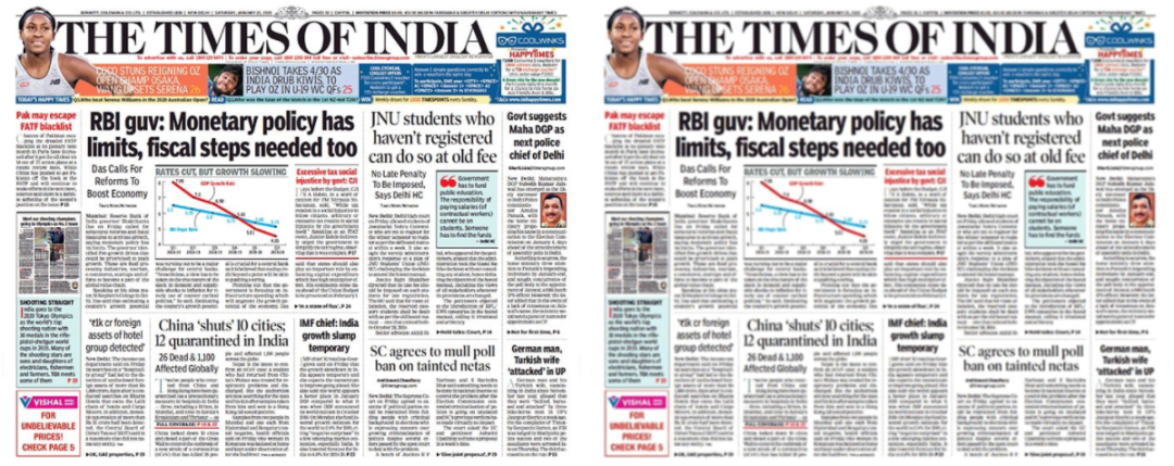
原始VS高斯模糊

阈 值

在图像处理中，阈值分割是最简单的图像分割方法，在灰度图像中，阈值可用于创建二值图像，这样做通常是为了清楚地区分不同的像素强度阴影。

简单阈值——如果像素值大于阈值，则为其分配一个值（可能是白色），否则为其分配另一个值（可能是黑色）。

自适应阈值——算法计算图像小区域的阈值。因此，对于同一图像的不同区域，我们可以得到不同的阈值，对于不同照明的图像，我们可以得到更好的结果。

注意：切记在阈值之前将图像转换为灰度

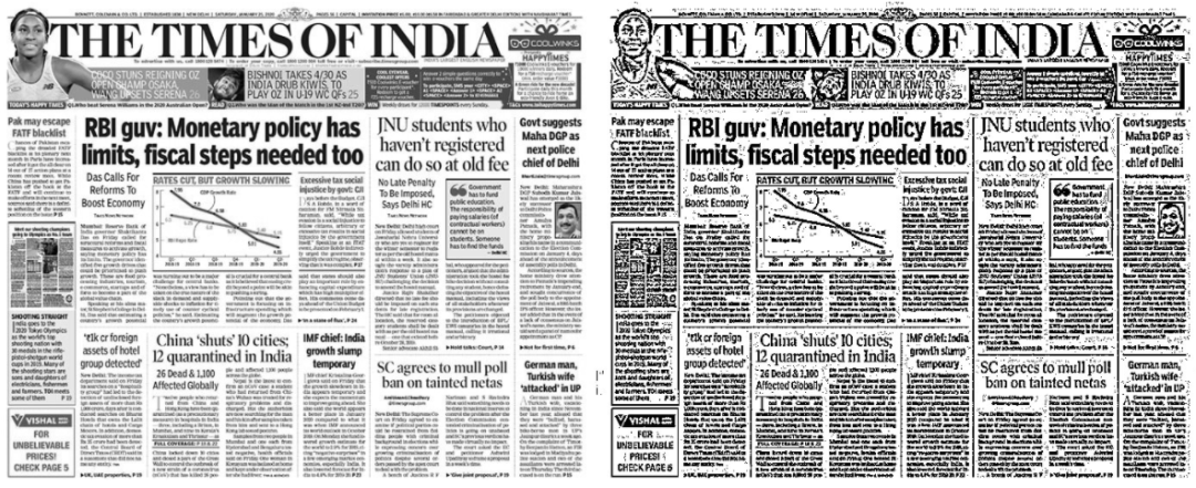
原始vs自适应高斯上的灰度缩放

去 噪

我们还进行了另一种去噪——非局部均值去噪。最初的去噪方法的原理是用附近像素颜色的平均颜色代替像素的颜色，概率论中的方差定律确保如果对 9 个像素求平均值，则平均值的噪声标准偏差除以 3。但是如果有边缘或拉长的图案，则通过平均去噪是不起作用的。因此，我们需要扫描图像的很大一部分，以搜索与我们想要去噪的像素真正相似的所有像素，然后通过计算这些最相似像素的平均颜色来完成去噪，这称为——非局部均值去噪。

使用cv2.fastNlMeans对其进行降噪。

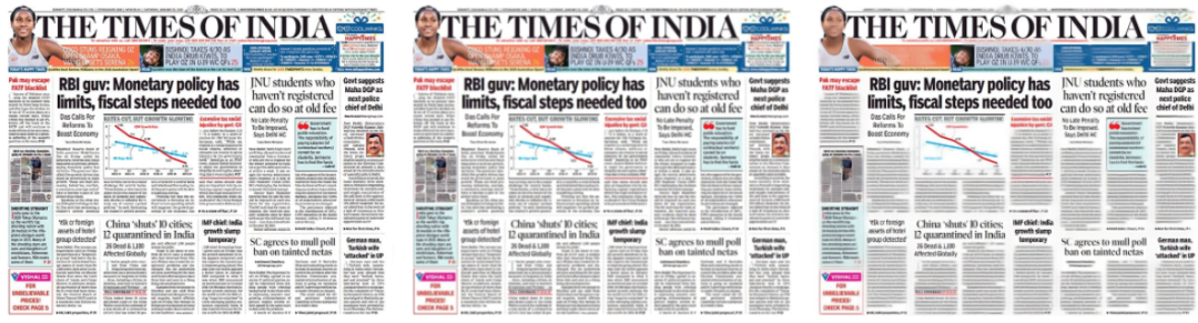
原始 vs 高斯模糊 vs 非局部均值去噪

Canny 边缘检测和最大轮廓提取

图像模糊和阈值处理之后，下一步是找到最大的轮廓（最大的边界框）并裁剪出图，这是通过使用 Canny 边缘检测然后使用四点变换提取最大轮廓来完成的。

Canny 边缘检测

Canny 边缘检测是一种多步骤的边缘检测算法，我们应该将去噪后的图像发送给该算法，以便它只能检测相关的边缘。

查找轮廓

找到边缘后，通过cv2.findcontours()传递图像，它连接所有具有相同颜色或强度的连续点（沿边缘），在此之后，我们将获得所有轮廓——矩形、球体等。

使用cv2.convexHull()和cv2.approxPolyDP找到照片中最大的矩形轮廓（大约）。

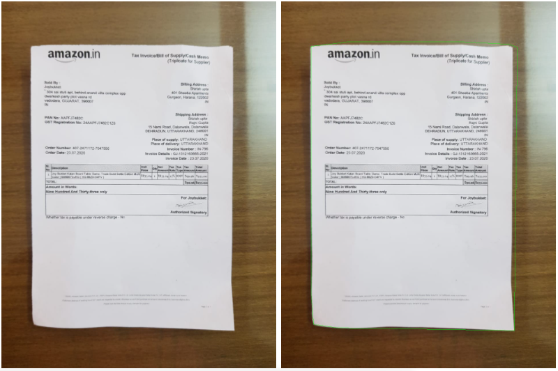
原始图像vs具有最大边界框的原始图像

提取最大的轮廓

虽然我们已经找到了看起来像矩形的最大轮廓，但我们仍然需要找到角点，以便找到裁剪图像的精确坐标。

首先，传递近似矩形（最大轮廓）的坐标，并在其上应用顺序点变换，结果是最大轮廓的精确 (x,y) 坐标。

四点变换——使用上面的 (x,y) 坐标，计算轮廓的宽度和高度，通过cv2.warpPerspective()来裁剪轮廓，下图表明我们已经成功地从输入图像中裁剪出相关数据了。

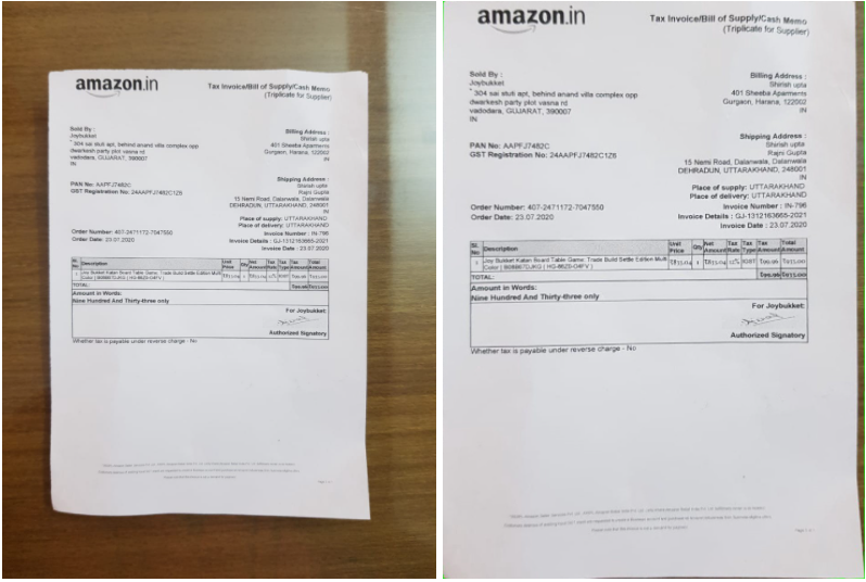
原始图像vs裁剪图像

最后——锐化和亮度校正

现在我们已经从图像中裁剪出相关信息（最大轮廓），最后一步是锐化图片，以便我们获得清晰可读的文档。

为此，我们使用色调、饱和度、值 (h,s,v)概念，其中值表示亮度，可以使用此值来增加文档的亮度。

—内核锐化 -内核、卷积矩阵或掩码是一个小矩阵，它用于模糊、锐化、浮雕、边缘检测等，这是通过在内核和图像之间进行卷积来实现的。

结果

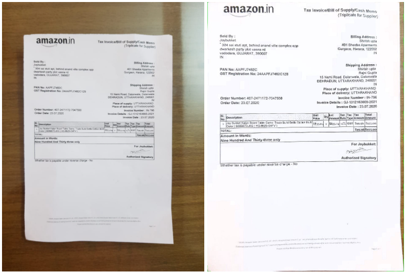
原始图像vs最终结果图像（裁剪、增亮和锐化）

完整代码

这是最终的代码

import numpy as np
import cv2
import re
from matplotlib import pyplot as plt




path = "/Users/shirishgupta/Desktop/ComputerVision/"
image = cv2.imread("/Users/shirishgupta/Desktop/ComputerVision/sample_image2.jpeg")




# ## **Use Gaussian Blurring combined with Adaptive Threshold** 


def blur_and_threshold(gray):
    gray = cv2.GaussianBlur(gray,(3,3),2)
    threshold = cv2.adaptiveThreshold(gray,255,cv2.ADAPTIVE_THRESH_GAUSSIAN_C, cv2.THRESH_BINARY,11,2)
    threshold = cv2.fastNlMeansDenoising(threshold, 11, 31, 9)
    return threshold




# ## **Find the Biggest Contour** 


# **Note: We made sure the minimum contour is bigger than 1/10 size of the whole picture. This helps in removing very small contours (noise) from our dataset**




def biggest_contour(contours,min_area):
    biggest = None
    max_area = 0
    biggest_n=0
    approx_contour=None
    for n,i in enumerate(contours):
            area = cv2.contourArea(i)




            if area > min_area/10:
                    peri = cv2.arcLength(i,True)
                    approx = cv2.approxPolyDP(i,0.02*peri,True)
                    if area > max_area and len(approx)==4:
                            biggest = approx
                            max_area = area
                            biggest_n=n
                            approx_contour=approx




    return biggest_n,approx_contour




def order_points(pts):
    # initialzie a list of coordinates that will be ordered
    # such that the first entry in the list is the top-left,
    # the second entry is the top-right, the third is the
    # bottom-right, and the fourth is the bottom-left
    pts=pts.reshape(4,2)
    rect = np.zeros((4, 2), dtype = "float32")


    # the top-left point will have the smallest sum, whereas
    # the bottom-right point will have the largest sum
    s = pts.sum(axis = 1)
    rect[0] = pts[np.argmin(s)]
    rect[2] = pts[np.argmax(s)]


    # now, compute the difference between the points, the
    # top-right point will have the smallest difference,
    # whereas the bottom-left will have the largest difference
    diff = np.diff(pts, axis = 1)
    rect[1] = pts[np.argmin(diff)]
    rect[3] = pts[np.argmax(diff)]


    # return the ordered coordinates
    return rect




# ## Find the exact (x,y) coordinates of the biggest contour and crop it out




def four_point_transform(image, pts):
    # obtain a consistent order of the points and unpack them
    # individually
    rect = order_points(pts)
    (tl, tr, br, bl) = rect


    # compute the width of the new image, which will be the
    # maximum distance between bottom-right and bottom-left
    # x-coordiates or the top-right and top-left x-coordinates
    widthA = np.sqrt(((br[0] - bl[0]) ** 2) + ((br[1] - bl[1]) ** 2))
    widthB = np.sqrt(((tr[0] - tl[0]) ** 2) + ((tr[1] - tl[1]) ** 2))
    maxWidth = max(int(widthA), int(widthB))




    # compute the height of the new image, which will be the
    # maximum distance between the top-right and bottom-right
    # y-coordinates or the top-left and bottom-left y-coordinates
    heightA = np.sqrt(((tr[0] - br[0]) ** 2) + ((tr[1] - br[1]) ** 2))
    heightB = np.sqrt(((tl[0] - bl[0]) ** 2) + ((tl[1] - bl[1]) ** 2))
    maxHeight = max(int(heightA), int(heightB))


    # now that we have the dimensions of the new image, construct
    # the set of destination points to obtain a "birds eye view",
    # (i.e. top-down view) of the image, again specifying points
    # in the top-left, top-right, bottom-right, and bottom-left
    # order
    dst = np.array([
        [0, 0],
        [maxWidth - 1, 0],
        [maxWidth - 1, maxHeight - 1],
        [0, maxHeight - 1]], dtype = "float32")


    # compute the perspective transform matrix and then apply it
    M = cv2.getPerspectiveTransform(rect, dst)
    warped = cv2.warpPerspective(image, M, (maxWidth, maxHeight))


    # return the warped image
    return warped




# # Transformation the image


# **1. Convert the image to grayscale**


# **2. Remove noise and smoothen out the image by applying blurring and thresholding techniques**


# **3. Use Canny Edge Detection to find the edges**


# **4. Find the biggest contour and crop it out**




def transformation(image):
  image=image.copy()  
  height, width, channels = image.shape
  gray=cv2.cvtColor(image,cv2.COLOR_BGR2GRAY)
  image_size=gray.size


  threshold=blur_and_threshold(gray)
  # We need two threshold values, minVal and maxVal. Any edges with intensity gradient more than maxVal 
  # are sure to be edges and those below minVal are sure to be non-edges, so discarded. 
  #  Those who lie between these two thresholds are classified edges or non-edges based on their connectivity.
  # If they are connected to "sure-edge" pixels, they are considered to be part of edges. 
  #  Otherwise, they are also discarded
  edges = cv2.Canny(threshold,50,150,apertureSize = 7)
  contours, hierarchy = cv2.findContours(edges, cv2.RETR_EXTERNAL, cv2.CHAIN_APPROX_SIMPLE)
  simplified_contours = []




  for cnt in contours:
      hull = cv2.convexHull(cnt)
      simplified_contours.append(cv2.approxPolyDP(hull,
                                0.001*cv2.arcLength(hull,True),True))
  simplified_contours = np.array(simplified_contours)
  biggest_n,approx_contour = biggest_contour(simplified_contours,image_size)


  threshold = cv2.drawContours(image, simplified_contours ,biggest_n, (0,255,0), 1)


  dst = 0
  if approx_contour is not None and len(approx_contour)==4:
      approx_contour=np.float32(approx_contour)
      dst=four_point_transform(threshold,approx_contour)
  croppedImage = dst
  return croppedImage




# **Increase the brightness of the image by playing with the "V" value (from HSV)**


def increase_brightness(img, value=30):
    hsv = cv2.cvtColor(img, cv2.COLOR_BGR2HSV)
    h, s, v = cv2.split(hsv)
    lim = 255 - value
    v[v > lim] = 255
    v[v <= lim] += value
    final_hsv = cv2.merge((h, s, v))
    img = cv2.cvtColor(final_hsv, cv2.COLOR_HSV2BGR)
    return img  




# **Sharpen the image using Kernel Sharpening Technique**




def final_image(rotated):
  # Create our shapening kernel, it must equal to one eventually
  kernel_sharpening = np.array([[0,-1,0], 
                                [-1, 5,-1],
                                [0,-1,0]])
  # applying the sharpening kernel to the input image & displaying it.
  sharpened = cv2.filter2D(rotated, -1, kernel_sharpening)
  sharpened=increase_brightness(sharpened,30)  
  return sharpened




# ## 1. Pass the image through the transformation function to crop out the biggest contour


# ## 2. Brighten & Sharpen the image to get a final cleaned image


blurred_threshold = transformation(image)
cleaned_image = final_image(blurred_threshold)
cv2.imwrite(path + "Final_Image2.jpg", cleaned_image)

下载1：OpenCV-Contrib扩展模块中文版教程

在「小白学视觉」公众号后台回复：扩展模块中文教程，即可下载全网第一份OpenCV扩展模块教程中文版，涵盖扩展模块安装、SFM算法、立体视觉、目标跟踪、生物视觉、超分辨率处理等二十多章内容。

下载2：Python视觉实战项目52讲

在「小白学视觉」公众号后台回复：Python视觉实战项目，即可下载包括图像分割、口罩检测、车道线检测、车辆计数、添加眼线、车牌识别、字符识别、情绪检测、文本内容提取、面部识别等31个视觉实战项目，助力快速学校计算机视觉。

下载3：OpenCV实战项目20讲

在「小白学视觉」公众号后台回复：OpenCV实战项目20讲，即可下载含有20个基于OpenCV实现20个实战项目，实现OpenCV学习进阶。

交流群

欢迎加入公众号读者群一起和同行交流，目前有SLAM、三维视觉、传感器、自动驾驶、计算摄影、检测、分割、识别、医学影像、GAN、算法竞赛等微信群（以后会逐渐细分），请扫描下面微信号加群，备注：”昵称+学校/公司+研究方向“，例如：”张三 + 上海交大 + 视觉SLAM“。请按照格式备注，否则不予通过。添加成功后会根据研究方向邀请进入相关微信群。请勿在群内发送广告，否则会请出群，谢谢理解~