此笔记用于分布式鲁棒优化入门。后续理论介绍均来源于这篇2025最新的DRO综述，非常不错。

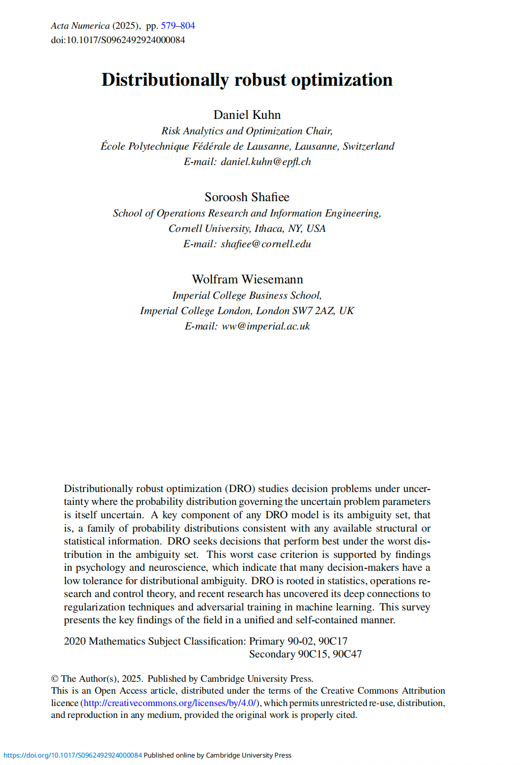
首先让我们来区分一下随机规划，鲁棒优化和分布式鲁棒优化。

Stochastic Programming (SP) 随机规划：

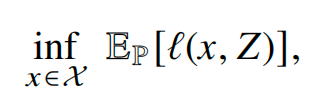
which explicitly model the uncertain problem parameters 𝑍 as a random vector that is governed by a probability distribution P, and where a decision is sought that performs best in expectation (or, subsequently, according to some risk measure).

Robust Optimization (RO)鲁棒优化：

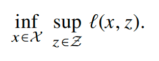
Robust optimization replaces the probabilistic description of the uncertain problem parameters with a set-based description and seeks for decisions that perform best in view of the worst anticipated parameter realization 𝑧 from within an uncertainty set Z. 

Distributionally Robust Optimization (DRO)分布式鲁棒优化：

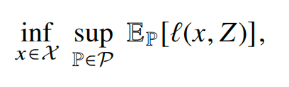
which model the uncertain problem parameters 𝑍 as a random vector that is governed by some distribution P from within an ambiguity set P, and where a decision is sought that performs best in view of its expected value under the worst distribution P ∈ P.

下面举一个常用的预测例子附代码来说明三者的区别。

Example: historical multivariate demand features X -> predict next-period demand y

1) Stochastic Programming (SP) / ERM:

   - Assume the empirical distribution is correct.

   - Minimize average loss on historical samples.

白话解释：就正常做预测那一套。

2) Robust Optimization (RO):

   - Ignore probabilities; protect against worst-case *scenario* among observed samples.

   - Minimize the maximum loss over samples (min–max).

白话解释：鲁棒优化不是在和某条固定的坏样本较劲，而是在找一个参数 w，让这个坏样本，坏得不至于太离谱。

3) Distributionally Robust Optimization (DRO):

   - Assume that the true distribution Q can only redistribute probabilities on these historical samples.

- Maximizes the average loss of the model by choosing one of the weight allocation methods (Choose the worst distribution).

- Minimize the above loss (min–max).

白话解释：看你怎么构造ambiguity,这里采用改变概率权重，还可以用KL / φ改概率，但受散度约束，用Wasserstein让样本可以“搬家”等等。找一个模型，使得即便未来把训练样本“按最坏方式重新加权”（每个样本权重最多），加权平均平方误差也尽可能小。

import numpy as np
import cvxpy as cp
from sklearn.model_selection import train_test_split
from sklearn.metrics import mean_squared_error

# ----------------------------
# 0) Toy "historical demand" dataset
# ----------------------------
rng = np.random.default_rng(0)
T, d = 300, 6
X = rng.normal(size=(T, d))
true_w = rng.normal(size=d)
y = X @ true_w + 0.3 * rng.normal(size=T)
outlier_idx = rng.choice(T, size=12, replace=False)
y[outlier_idx] += rng.normal(loc=0.0, scale=6.0, size=len(outlier_idx))
y = y.reshape(-1, 1)

X_train, X_test, y_train, y_test = train_test_split(X, y, test_size=0.25, random_state=0)

# Add intercept
def add_intercept(X):
    return np.hstack([np.ones((X.shape[0], 1)), X])

Xtr = add_intercept(X_train)
Xte = add_intercept(X_test)
n, p = Xtr.shape

# ----------------------------
# 1) ERM (SP): average squared loss
# ----------------------------
w_erm = cp.Variable((p, 1))
obj_erm = cp.Minimize(cp.sum_squares(y_train - Xtr @ w_erm) / n)
cp.Problem(obj_erm).solve(solver=cp.OSQP)
mse_erm = mean_squared_error(y_test, Xte @ w_erm.value)


# ----------------------------
# 2) RO: minimize worst sample squared loss
# ----------------------------
w_ro = cp.Variable((p, 1))
t = cp.Variable(nonneg=True)
res = y_train - Xtr @ w_ro
constraints_ro = [cp.square(res[i, 0]) <= t for i in range(n)]
cp.Problem(cp.Minimize(t), constraints_ro).solve(solver=cp.ECOS)
mse_ro = mean_squared_error(y_test, Xte @ w_ro.value)

# ----------------------------
# 3) DRO (explicit): reweighting ambiguity set + LP dual
#
#   min_w  max_q  sum_i q_i * loss_i(w)
#   s.t.   q in simplex, and q_i <= q_max
#
# Dual form:
#   min_{w, alpha, beta>=0}  alpha + q_max * sum_i beta_i
#   s.t. alpha + beta_i >= loss_i(w)
# ----------------------------

eps = 0.8                 # robustness level (bigger => more adversarial reweighting)
q_max = (1 + eps) / n     # each sample weight capped

w_dro = cp.Variable((p, 1))
alpha = cp.Variable()                 # dual scalar
beta = cp.Variable((n, 1), nonneg=True)

loss = cp.square(y_train - Xtr @ w_dro)   # elementwise squared residuals (n x 1)

constraints_dro = [
    alpha + beta >= loss
]

obj_dro = cp.Minimize(alpha + q_max * cp.sum(beta))
cp.Problem(obj_dro, constraints_dro).solve(solver=cp.ECOS)

mse_dro = mean_squared_error(y_test, Xte @ w_dro.value)

print("Test MSE (lower is better):")
print(f"  ERM (avg loss):                 {mse_erm:.4f}")
print(f"  RO  (worst single sample):      {mse_ro:.4f}")
print(f"  DRO (worst reweighted average): {mse_dro:.4f}")
    

How to read results:

- ERM: fits the average behavior; can be sensitive to outliers / mis-specified distribution.

- RO : tries to reduce the worst-case training error; can become conservative (may underfit).

- DRO : sits between: more robust than ERM, often less conservative than RO; rho controls robustness.