import pandas as pd
import numpy as np
import matplotlib.pyplot as plt
import seaborn as sns


from sklearn.decomposition import PCA


from sklearn.svm import SVC
from sklearn.tree import DecisionTreeClassifier
from sklearn.metrics import confusion_matrix, ConfusionMatrixDisplay,classification_report,accuracy_score
from sklearn.ensemble import RandomForestClassifier
from sklearn.neighbors import KNeighborsClassifier
from sklearn.naive_bayes import GaussianNB
from sklearn.linear_model import LogisticRegression
from sklearn.preprocessing import StandardScaler
from sklearn.model_selection import train_test_split,cross_val_score,KFold,ShuffleSplit


import pickle


# Codes for good plots
plt.rcParams.update({'font.size':14})
plt.rcParams.update({"font.family" : "Times new roman"})
column_names = ['Time', 'Ipv', 'Vpv', 'Vdc', 'ia', 'ib', 'ic', 'va', 'vb', 'vc', 'Iabc',
       'If', 'Vabc', 'Vf', 'label']
solar_data_Lim_power=pd.DataFrame(columns = column_names)
solar_data_Max_power=pd.DataFrame(columns = column_names)
for num in range(0,8): 
    df = pd.read_csv(r'CSV_Files\F{}L.csv'.format(num))
    df['label']=np.full((len(df),1),'F{}L'.format(num))
    solar_data_Lim_power=pd.concat([solar_data_Lim_power, df], ignore_index=True)
    
    df1 = pd.read_csv(r'CSV_Files\F{}M.csv'.format(num))
    df1['label']=np.full((len(df1),1),'F{}M'.format(num))
    solar_data_Max_power=pd.concat([solar_data_Max_power, df1], ignore_index=True)
solar_data_Lim_power.head()

solar_data_Max_power.head()

solar_data_Lim_power1= solar_data_Lim_power.iloc[::1000,:]
for col in solar_data_Lim_power1.columns[1:-1]:
    fig = plt.figure(figsize=(5,5))
    sns.scatterplot(data=solar_data_Lim_power1, x="Time", y=col,hue="label",style="label",palette='viridis',edgecolor="white",s=100)
    plt.xlabel('Time')
    plt.ylabel(col)
    plt.show()

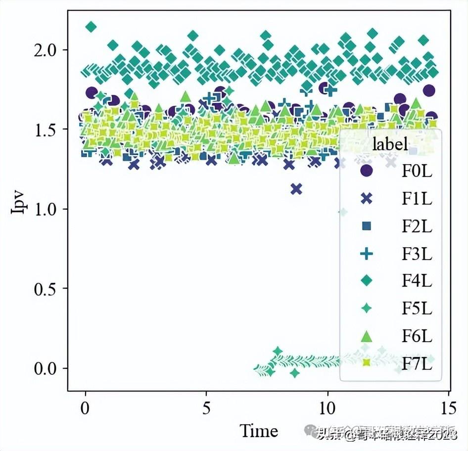
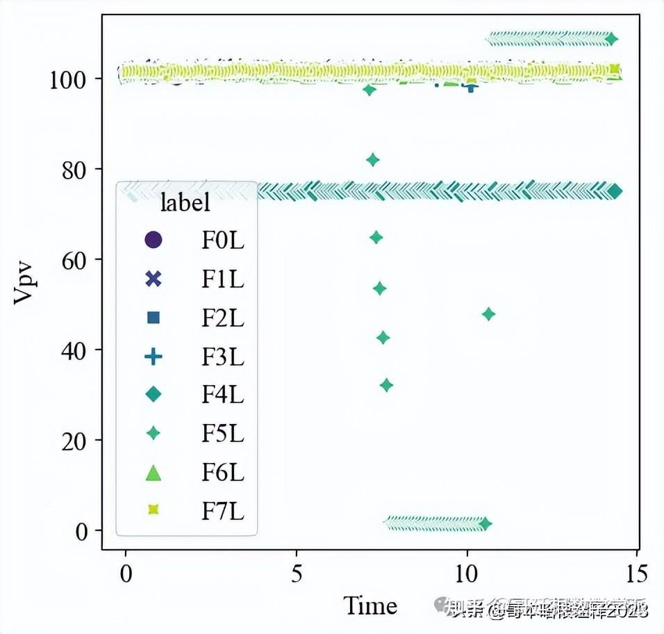
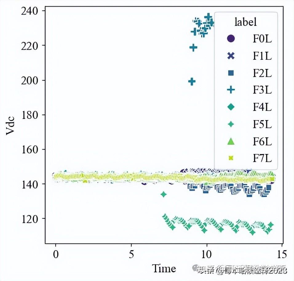
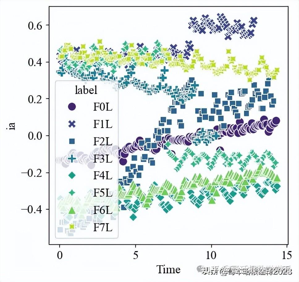
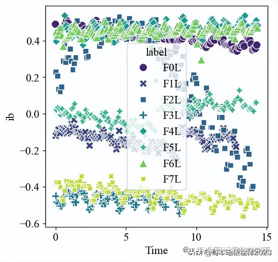
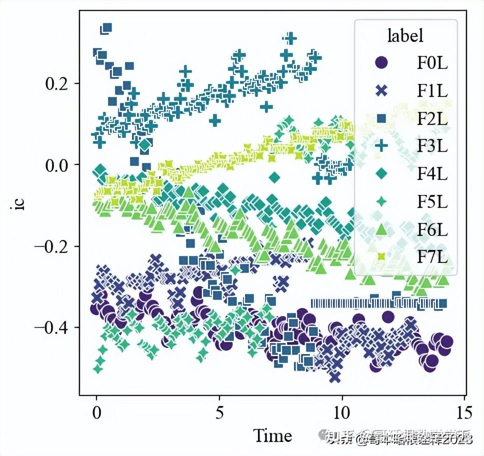
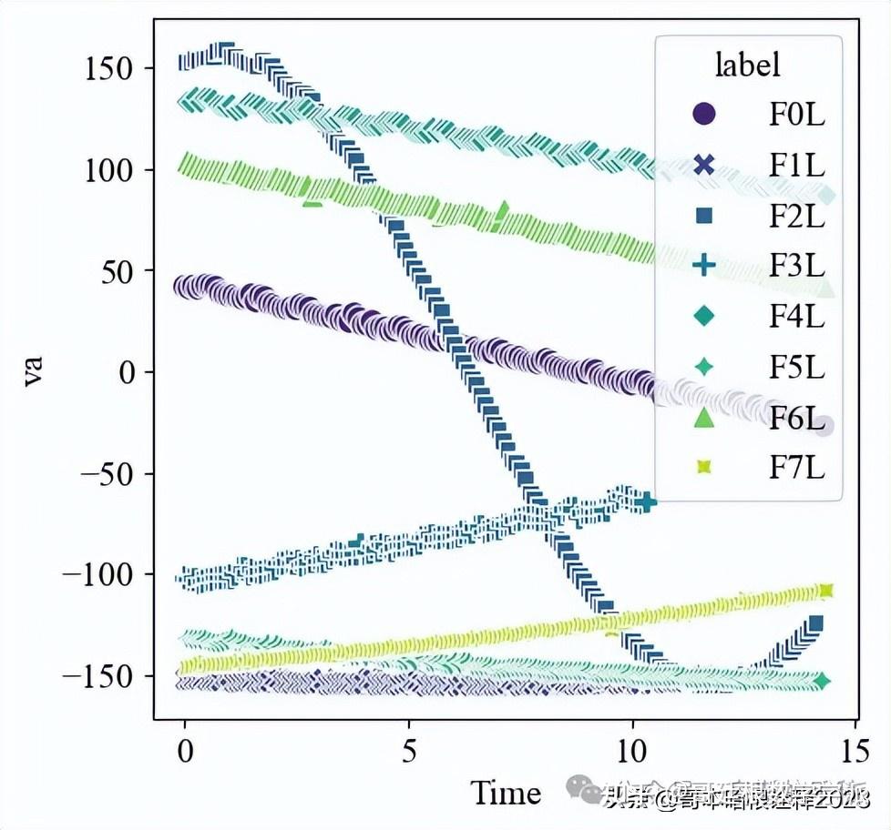
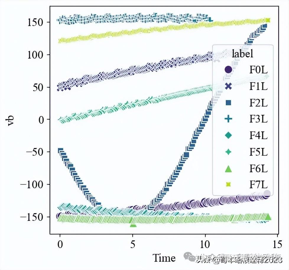
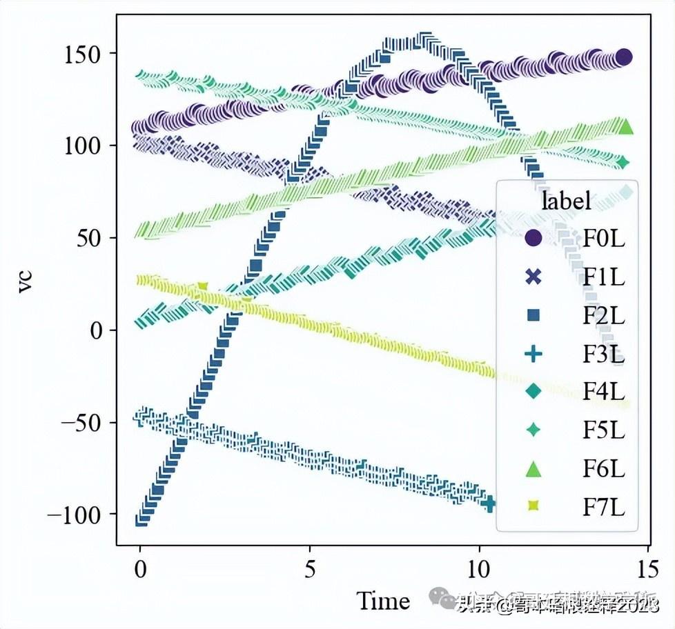
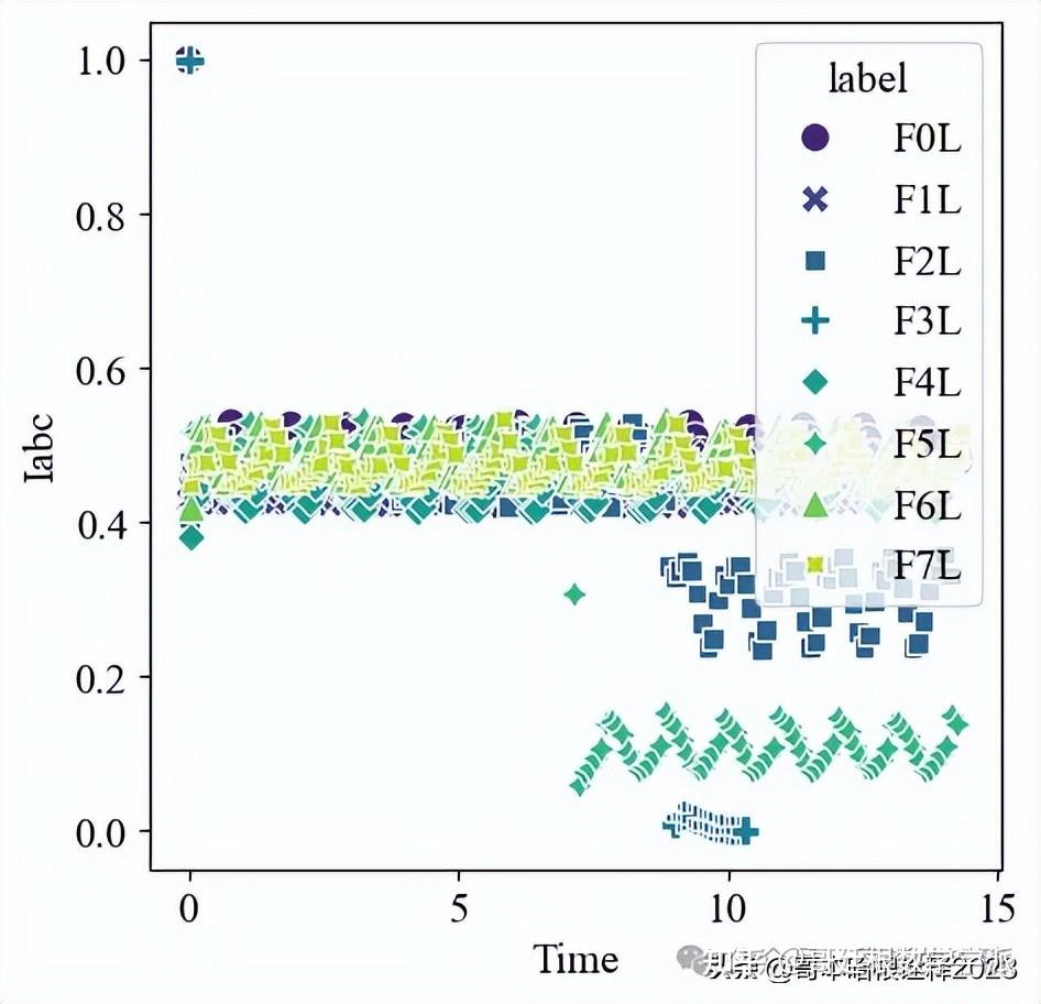
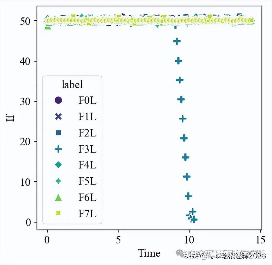
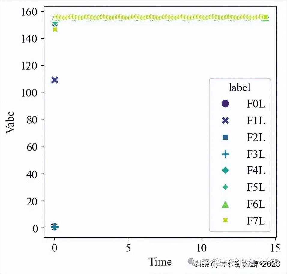
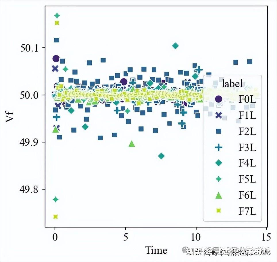
solar_data_Lim_power.iloc[::100,:].to_csv(r'Lim_solar_data.csv',index=False)
solar_data_Max_power.iloc[::100,:].to_csv(r'Max_solar_data.csv',index=False)

Import The Limited Power Dataset

df1=pd.read_csv(r'preprocessed_data\Lim_solar_data.csv')
df2=pd.read_csv(r'D:\py_projects\Solar panel fault diagnosis\preprocessed_data\Max_solar_data.csv')


df1.head()

df1.info()
<class 'pandas.core.frame.DataFrame'>
RangeIndex: 10935 entries, 0 to 10934
Data columns (total 15 columns):
 #   Column  Non-Null Count  Dtype  
---  ------  --------------  -----  
 0   Time    10935 non-null  float64
 1   Ipv     10935 non-null  float64
 2   Vpv     10935 non-null  float64
 3   Vdc     10935 non-null  float64
 4   ia      10935 non-null  float64
 5   ib      10935 non-null  float64
 6   ic      10935 non-null  float64
 7   va      10935 non-null  float64
 8   vb      10935 non-null  float64
 9   vc      10935 non-null  float64
 10  Iabc    10935 non-null  float64
 11  If      10935 non-null  float64
 12  Vabc    10935 non-null  float64
 13  Vf      10935 non-null  float64
 14  label   10935 non-null  object 
dtypes: float64(14), object(1)
memory usage: 1.3+ MB
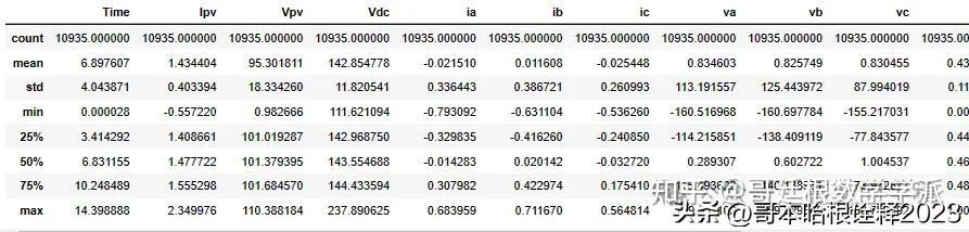
df1.describe()

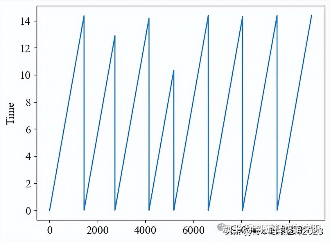
plt.plot(df1['Time'])
plt.ylabel('Time')
plt.show()

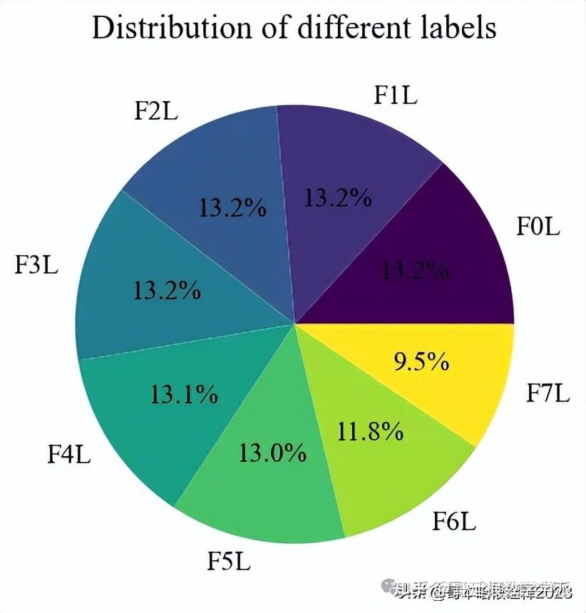
Pie Chart for samples from each fault class

df1['label'].value_counts()
label
F7L    1441
F4L    1440
F6L    1440
F0L    1438
F5L    1430
F2L    1421
F1L    1290
F3L    1035
Name: count, dtype: int64

X = df1.iloc[:,1:-1] #Features
Y = df1.iloc[:,-1]   #Traget Labels




plt.figure(figsize=(10,10))
sns.heatmap(X.corr(),annot=True,cmap='viridis')
plt.show()

Data Visualization

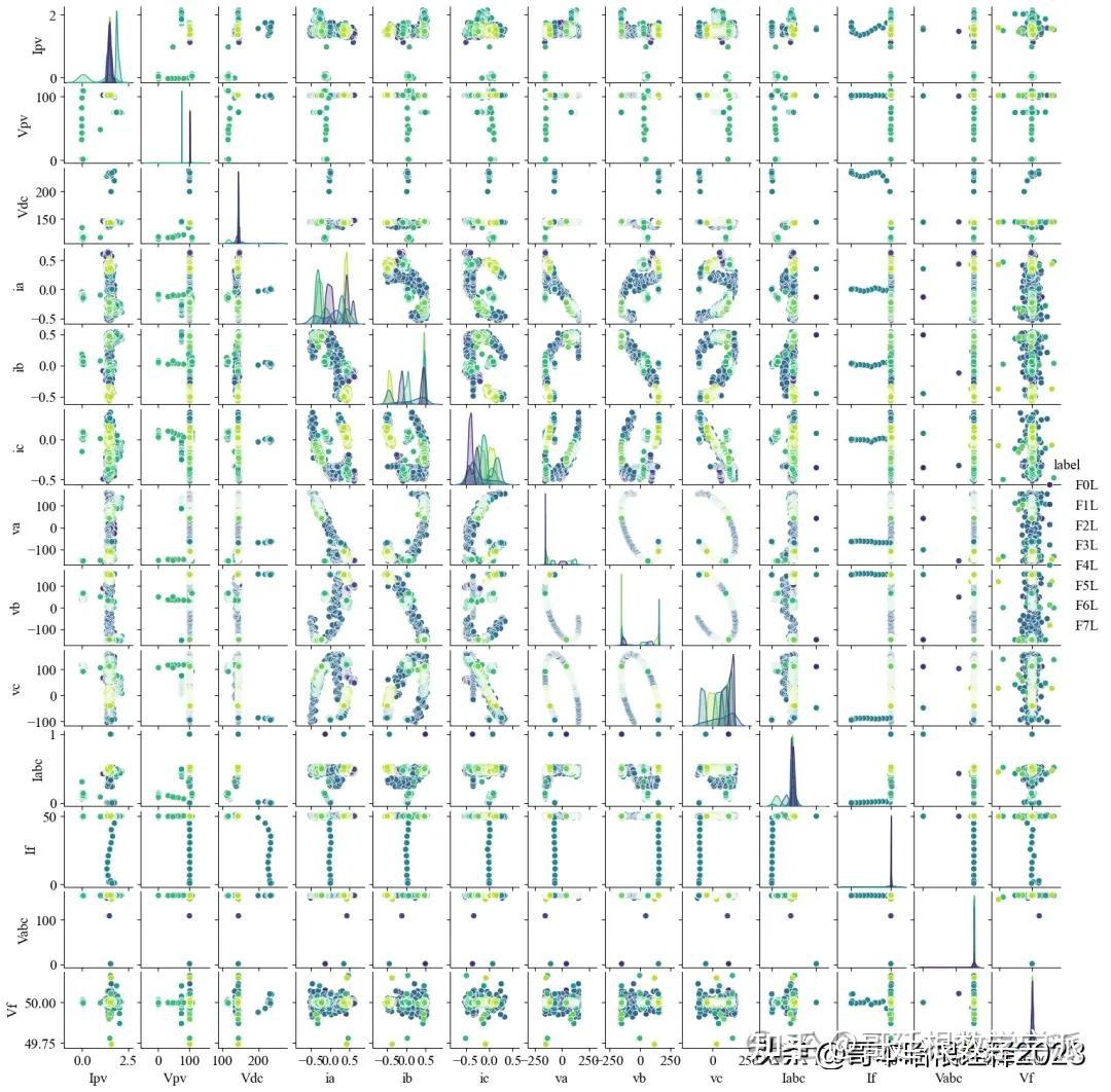
g=sns.pairplot(data=df1.iloc[::10,1:], hue="label",palette='viridis')
g.fig.set_size_inches(15,15)

Divide the dataset into Train-test split and do the standard scalling

X_train,X_test,y_train,y_test = train_test_split(X,Y,test_size=0.2,shuffle=True)


scaler=StandardScaler()
X_sc_train = scaler.fit_transform(X_train)
X_sc_test = scaler.transform(X_test)
print("The number of samples in the Training set is {}".format(len(X_train)))
print("The number of samples in the Test set is {}".format(len(X_test)))
The number of samples in the Training set is 8748
The number of samples in the Test set is 2187

Dimensionality Reduction Using PCA

pca = PCA(n_components=2)
pca.fit(X_sc_train)
PCA(n_components=2)
transformed = pca.transform(X_sc_train)
X_sc_train.shape
(8748, 13)
transformed
array([[-1.88480762, -0.71094237],
       [ 2.30202284, -0.52113464],
       [-1.90030091, -0.63863273],
       ...,
       [-1.02861664,  0.24289999],
       [ 2.05086121, -0.15209862],
       [ 2.09889048, -0.47981136]])
pca.explained_variance_ratio_
array([0.2748987, 0.1702507])
for i in range (1,14):
    pca = PCA(n_components=i)
    # prepare transform on dataset
    pca.fit(X_sc_train)
    # apply transform to dataset
    transformed = pca.transform(X_sc_train)
    print("Cummulative explained variance for {}-component: {} ".format(i,np.sum(pca.explained_variance_ratio_)))
    print("")
Cummulative explained variance for 1-component: 0.2748987018247871 

Cummulative explained variance for 2-component: 0.4451494028455815 

Cummulative explained variance for 3-component: 0.6066151451895915 

Cummulative explained variance for 4-component: 0.7422823834696191 

Cummulative explained variance for 5-component: 0.8220485218416997 

Cummulative explained variance for 6-component: 0.8964391080151923 

Cummulative explained variance for 7-component: 0.9548862398316027 

Cummulative explained variance for 8-component: 0.973025172997148 

Cummulative explained variance for 9-component: 0.9861755544237186 

Cummulative explained variance for 10-component: 0.993179519856309 

Cummulative explained variance for 11-component: 0.998235993441997 

Cummulative explained variance for 12-component: 0.9999865290966475 

Cummulative explained variance for 13-component: 1.0

PCA with 2 components Visualization

pca = PCA(n_components=2)
# prepare transform on dataset
pca.fit(X_sc_train)
# apply transform to dataset
transformed = pca.transform(X_sc_train)
#Make a data Frame
principalDf = pd.DataFrame(data = transformed
             , columns = ['principal component 1', 'principal component 2'])
# Plot the PC-1 and PC-2
fig, ax = plt.subplots(figsize=(7,7))
sns.scatterplot(x=principalDf['principal component 1'],y=principalDf['principal component 2'],hue=y_train,palette='viridis')
plt.show()

PCA with 3 components Visualization

pca_3 = PCA(n_components=3)


X_pca = pca_3.fit_transform(X_sc_train)


principalDf = pd.DataFrame(data = X_pca, columns = ['principal component 1', 'principal component 2','principal component 3'])


principalDf['Fault']=np.array(y_train)
from mpl_toolkits.mplot3d import Axes3D
%matplotlib qt




fig = plt.figure(figsize=(8,8))
  
# syntax for 3-D projection
ax = plt.axes(projection='3d')
  
# defining all 3 axes
fault = y_train.unique()
colors = ['g', 'r','b','y','c','m','k']
for fault, color in zip(fault,colors):
    indicesToKeep = principalDf['Fault'] == fault
    ax.scatter3D(principalDf.loc[indicesToKeep, 'principal component 1']
               , principalDf.loc[indicesToKeep, 'principal component 2']
               , principalDf.loc[indicesToKeep, 'principal component 3']
               , c = color
               , s = 50)
ax.legend(y_train.unique())


  
# plotting
ax.set_xlabel('Principal Component 1', fontsize = 15)
ax.set_ylabel('Principal Component 2', fontsize = 15)
ax.set_zlabel('Principal Component 3', fontsize = 15)


ax.set_title('3D PCA')
ax.view_init(45,90)


plt.show()

Combining Datasets

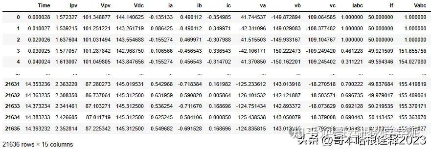
df = pd.concat([df1,df2], ignore_index=True, axis=0)
df

df['label'].unique()
array(['F0L', 'F1L', 'F2L', 'F3L', 'F4L', 'F5L', 'F6L', 'F7L', 'F0M',
       'F1M', 'F2M', 'F3M', 'F4M', 'F5M', 'F6M', 'F7M'], dtype=object)

Divide the dataset into Train-test split and do the standard scalling

def split_transform(df,split_ratio):
    X=df.iloc[:,0:-1]
    Y=df.iloc[:,-1]
    X_train,X_test,y_train,y_test = train_test_split(X,Y,test_size=split_ratio,shuffle=True)


    scaler=StandardScaler()
    X_sc_train = scaler.fit_transform(X_train)
    X_sc_test = scaler.transform(X_test)


    print("The number of samples in the Training set is {}".format(len(X_sc_train)))
    print("The number of samples in the Test set is {}".format(len(X_sc_test)))
    
    return  X_sc_train, X_sc_test,y_train,y_test,scaler
X_sc_train, X_sc_test,y_train,y_test,scaler = split_transform(df,split_ratio=0.02)
The number of samples in the Training set is 21203
The number of samples in the Test set is 433

Model training

def Model_with_cross_val(df,clf,k_fold,test_size):
    # Split transform the data
    X_sc_train, X_sc_test,y_train,y_test,scaler = split_transform(df,split_ratio=0.01)
    print("")
    #Generate k-fold with shuffled split
    cv = ShuffleSplit(n_splits=k_fold, test_size=test_size)
    
    # get score for each split
    scores = cross_val_score(clf, X_sc_train,y_train, cv=cv, n_jobs=-1)
    
    #print scores with mean and std
    print(scores)
    
    print("{} accuracy with a standard deviation of {}".format(np.mean(scores),np.std(scores)))
    print("")
clf = RandomForestClassifier()
Model_with_cross_val(df=df,clf=clf,k_fold=5,test_size=0.3)
The number of samples in the Training set is 21419
The number of samples in the Test set is 217

[0.98910675 0.99330843 0.99112979 0.9929972  0.99268596]
0.9918456271397448 accuracy with a standard deviation of 0.0015611498542153093

Decision Trees

clf = DecisionTreeClassifier()
Model_with_cross_val(df=df,clf=clf,k_fold=5,test_size=0.3)
The number of samples in the Training set is 21419
The number of samples in the Test set is 217

[0.97261127 0.97525677 0.97603486 0.97385621 0.96794273]
0.9731403672580143 accuracy with a standard deviation of 0.0028518421883486724

SVM

clf = SVC()
Model_with_cross_val(df=df,clf=clf,k_fold=5,test_size=0.3)
The number of samples in the Training set is 21419
The number of samples in the Test set is 217

[0.96125117 0.96125117 0.96125117 0.96171802 0.9589169 ]
0.9608776844070961 accuracy with a standard deviation of 0.0009969260739525

KNN

clf = KNeighborsClassifier(n_neighbors=5)
Model_with_cross_val(df=df,clf=clf,k_fold=5,test_size=0.3)
The number of samples in the Training set is 21419
The number of samples in the Test set is 217

[0.96716464 0.96840959 0.96700903 0.96545285 0.96545285]
0.966697790227202 accuracy with a standard deviation of 0.0011264837267882745

Logistic Reg

clf = LogisticRegression()
Model_with_cross_val(df=df,clf=clf,k_fold=5,test_size=0.3)
The number of samples in the Training set is 21419
The number of samples in the Test set is 217

[0.7351385  0.74680984 0.74323063 0.75412387 0.75241208]
0.7463429816370992 accuracy with a standard deviation of 0.006823800722503431

prediction with best performing Model

X_sc_train, X_sc_test,y_train,y_test,scaler = split_transform(df,split_ratio=0.2)


Model = RandomForestClassifier()
Model.fit(X_sc_train,y_train)


fig, ax = plt.subplots(figsize=(10,10))
disp = ConfusionMatrixDisplay.from_estimator(
    Model,
    X_sc_test,
    y_test,
    display_labels=Model.classes_,
    cmap=plt.cm.Reds
)




disp.plot(ax=ax)
The number of samples in the Training set is 17308
The number of samples in the Test set is 4328
print("Random Forest")
clf_random_forest = RandomForestClassifier()
Model_with_cross_val(df=df,clf=clf_random_forest,k_fold=5,test_size=0.3)
print("")
print("Decision Tree")
clf_decision_tree = DecisionTreeClassifier()
Model_with_cross_val(df=df,clf=clf_decision_tree,k_fold=5,test_size=0.3)
print("")
print("Support Vector Machines")
clf = SVC()
Model_with_cross_val(df=df,clf=clf,k_fold=5,test_size=0.3)
print("")
print("KNN")
clf_knn = KNeighborsClassifier(n_neighbors=5)
Model_with_cross_val(df=df,clf=clf_knn,k_fold=5,test_size=0.3)
print("")
print("Logistic Regression")
clf = LogisticRegression()
Model_with_cross_val(df=df,clf=clf,k_fold=5,test_size=0.3)
print("")
print("Naive Byes")
clf = GaussianNB()
Model_with_cross_val(df=df,clf=clf,k_fold=5,test_size=0.3)
Random Forest
The number of samples in the Training set is 21419
The number of samples in the Test set is 217

[0.98770619 0.98910675 0.98506069 0.98786181 0.98957361]
0.9878618113912232 accuracy with a standard deviation of 0.0015716627666296098


Decision Tree
The number of samples in the Training set is 21419
The number of samples in the Test set is 217

[0.96903206 0.97136632 0.96560847 0.96949891 0.96981015]
0.9690631808278866 accuracy with a standard deviation of 0.001896750573942447


Support Vector Machines
The number of samples in the Training set is 21419
The number of samples in the Test set is 217

[0.90771864 0.91020853 0.90538438 0.91160909 0.90585123]
0.9081543728602552 accuracy with a standard deviation of 0.0024216450250765156


KNN
The number of samples in the Training set is 21419
The number of samples in the Test set is 217

[0.93713041 0.9291939  0.93697479 0.92950514 0.93059446]
0.9326797385620914 accuracy with a standard deviation of 0.0036009300477823107


Logistic Regression
The number of samples in the Training set is 21419
The number of samples in the Test set is 217

[0.57671958 0.5620915  0.58123249 0.56598195 0.56971678]
0.5711484593837535 accuracy with a standard deviation of 0.006978482517667545


Naive Byes
The number of samples in the Training set is 21419
The number of samples in the Test set is 217

[0.5751634  0.57796452 0.58527856 0.56053533 0.58356676]
0.5765017117958294 accuracy with a standard deviation of 0.008784125288306617

学术咨询：

担任《Mechanical System and Signal Processing》《中国电机工程学报》等期刊审稿专家，擅长领域：信号滤波/降噪，机器学习/深度学习，时间序列预分析/预测，设备故障诊断/缺陷检测/异常检测。

分割线分割线分割线

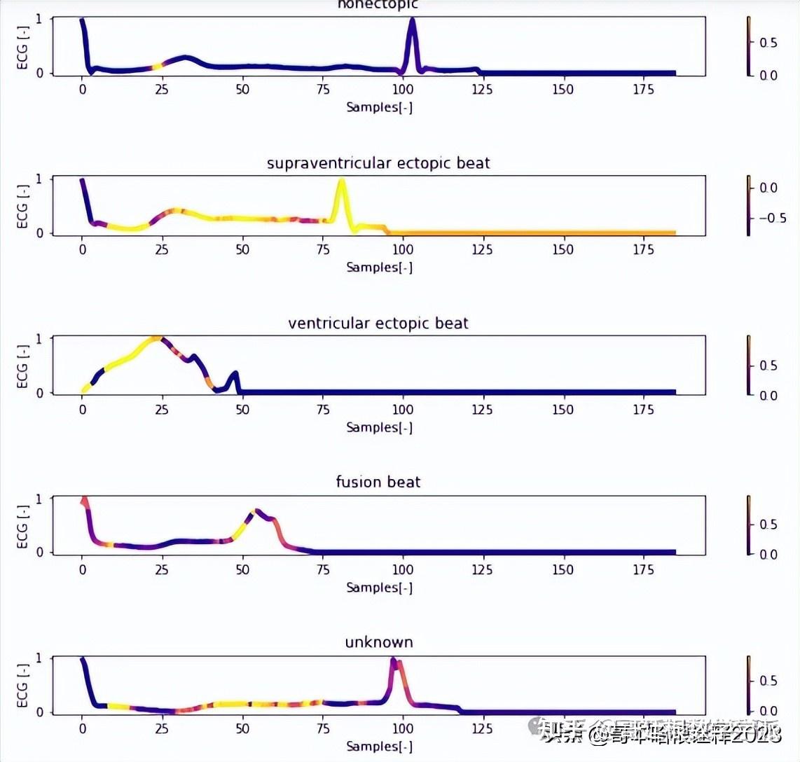
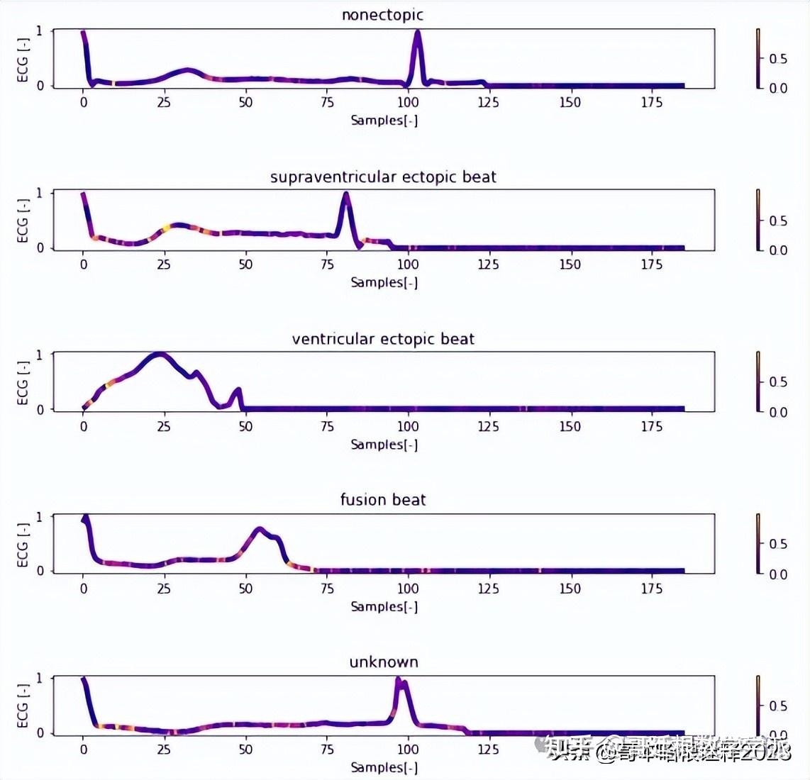
一维神经网络的特征可视化分析-以心电信号为例（Python，Jupyter Notebook）

包括Occlusion sensitivity方法，Saliency map方法，Grad-CAM方法

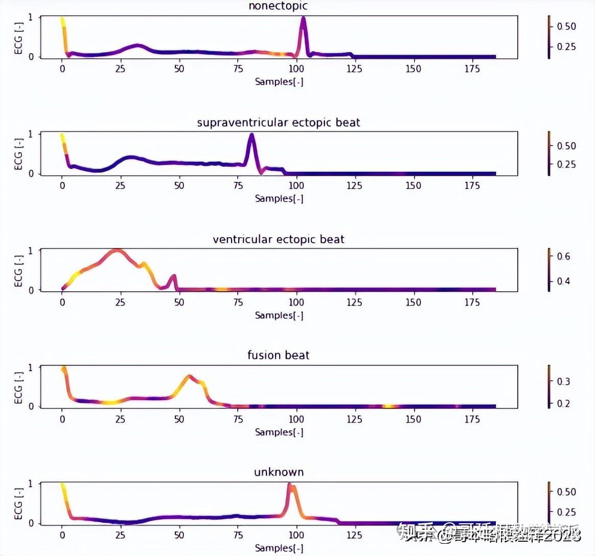
完整代码可通过学术咨询获得：

基于深度学习的机械故障诊断及其权重可视化（Python）

医学图像的深度学习可解释性（MATLAB R2021B）

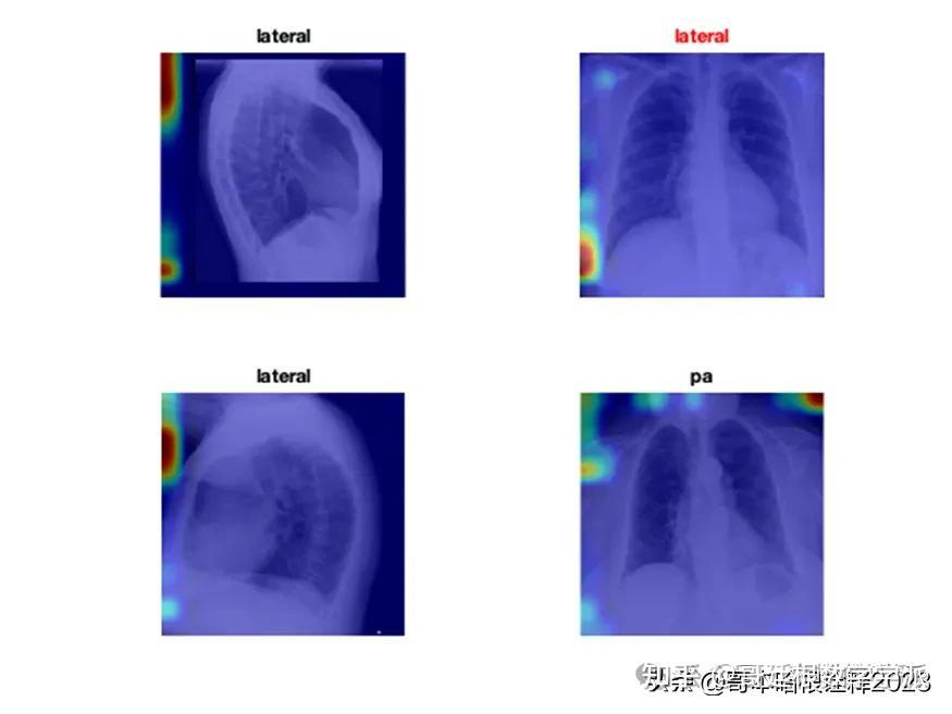
完整代码可通过学术咨询获得：

一维时间序列信号的稀疏度度量方法（MATLAB R2018A）

算法运行环境为MATLAB R2018A，执行一维信号的稀疏度量方法，包括峰度(Kurt)、负熵(NE)、d -范数(DN)、2-范数与1-范数之比(L2/L1)、基尼指数(GI)、修正平滑指数(MSI)、基尼指数2 (GI2)、基尼指数3 (GI3)、广义基尼指数(GGI)、完全广义基尼指数等。

算法可迁移至金融时间序列，地震信号，机械振动信号，语音信号，声信号，生理信号（EEG,EMG）等一维时间序列信号。

基于脉冲小波的旋转机械故障诊断（MATLAB R2018a）

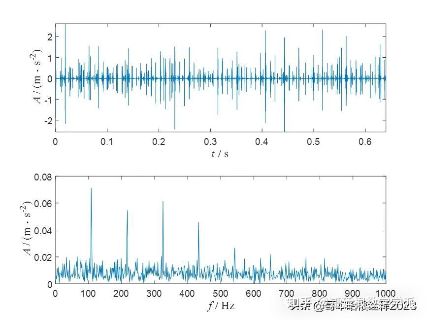
完整代码可通过学术咨询获得：

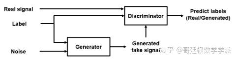
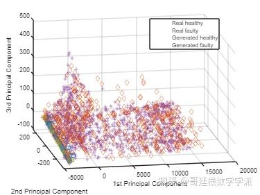
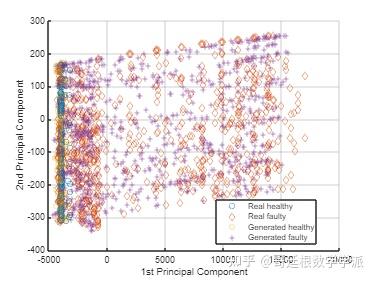
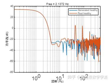
使用条件生成对抗网络CGAN生成三缸泵流量信号（MATLAB R2021B）