实验内容：

1. 编码实现基于最小二乘法的单变量线性回归算法

最小二乘法是一种数学优化技术，通过最小化误差的平方和来找到数据的最佳函数匹配。在单变量线性回归中找到一条直线 𝑦=𝑤𝑥+𝑏，使得该直线与数据集中的点的垂直距离的平方和最小。

算法步骤：

1. 计算 x 和 y 的均值
2. 计算斜率 𝑤
3. 计算截距 𝑏
4. 使用 𝑤 和 𝑏 来预测新的 y 值

（2）画数据散点图，以及得到的直线

绘图步骤：

1. 使用 scatter 函数绘制原始数据点。
2. 使用 plot 函数绘制拟合直线。
3. 添加图例、标签和标题。

基于训练得到的参数，输入新的样本数据，输出预测值；

实验结果：

（1）以下是使用最小二乘法实现的单变量线性回归算法的代码

'''
Author: Yeechen
Description:  Single variable linear regression algorithm implemented using least squares method
'''

import matplotlib.pyplot as plt
import numpy as np

# Load data from a text file
points = np.loadtxt("data.txt", delimiter=',')
x = points[:, 0]
y = points[:, 1]

# Calculate the mean of a dataset
def calculate_mean(data):
    return np.mean(data)

# Calculate the sum of a dataset
def sum_x(data):
    return np.sum(data)

# Calculate the sum of the square of a dataset
def sum_x_squared(data):
    return np.sum(data ** 2)

# Calculate the sum of the product of (x - x_mean) and y
def sum_xy(points):
    x_bar = calculate_mean(points[:, 0])
    return np.sum(points[:, 1] * (points[:, 0] - x_bar))

# Calculate the weight (w) for the linear regression line
def calculate_w(points):
    m = len(points)
    numerator = sum_xy(points)
    denominator = sum_x_squared(points[:, 0]) - (sum_x(points[:, 0]) ** 2) / m
    if denominator == 0:
        return 0
    else:
        return numerator / denominator

# Calculate the y-intercept (b) for the linear regression line
def calculate_b(y, w, x_mean):
    return calculate_mean(y) - w * x_mean

# Predict y values using the linear regression equation
def predict_y(x, w, b):
    return w * x + b

w = calculate_w(points)
x_mean = calculate_mean(x)
b = calculate_b(y, w, x_mean)

# Predict y values using the calculated weight and y-intercept
pred_y = predict_y(x, w, b)

# Plot the original data points and the linear fit line
plt.scatter(x, y, label='Data Points')
plt.plot(x, pred_y, color='red', label='Linear Fit')
plt.xlabel('X')
plt.ylabel('Y')
plt.legend()
plt.show()

（2）基于代码实现，所得数据散点图和拟合直线如图1所示：

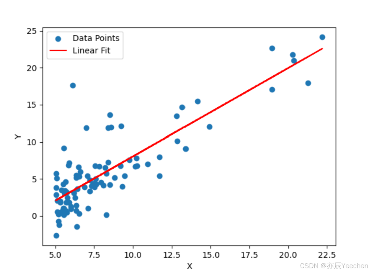
图1 数据散点图和拟合直线

（3）假设有新的样本数据 𝑥𝑛𝑒𝑤​，我们可以使用训练得到的模型参数 𝑤 和 𝑏 来预测 𝑦𝑛𝑒𝑤。使用Jupyter Notebook进行新样本数据的预测，由上可得拟合直线的 𝑤 和 𝑏 分别为1.193和-3.896，现假设新样本数据 𝑥𝑛𝑒𝑤 分别为5和10，可得到拟合值 𝑦𝑛𝑒𝑤 如图2所示：

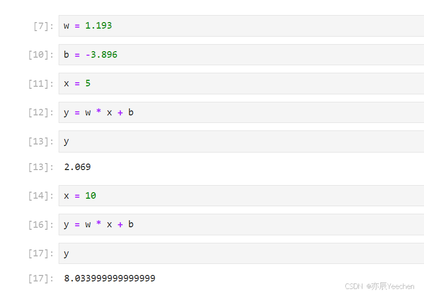
图2 基于拟合直线进行新样本数据预测的结果