python求解常见的最优化问题

多变量最优化
问题：
彩电商准备推出两种产品，19寸彩电，建议价格339美元（成本195美元），21寸彩电，建议价格399美元（成本225美元），
固定成本400000美元，已知每售出一台彩电，会导致彩电价格下降1美分，而且每售出一台19寸彩电，会导致21寸彩电下降0.4美分；
每售出一台21寸彩电，会导致19寸彩电下降0.3美分，请问每台彩电应该生产多少台才能达到最大收益。

from sympy import *
from sympy.plotting import plot3d

"""
多变量最优化
问题：
彩电商准备推出两种产品，19寸彩电，建议价格339美元（成本195美元），21寸彩电，建议价格399美元（成本225美元），
固定成本400000美元，已知每售出一台彩电，会导致彩电价格下降1美分，而且每售出一台19寸彩电，会导致21寸彩电下降0.4美分；
每售出一台21寸彩电，会导致19寸彩电下降0.3美分，请问每台彩电应该生产多少台才能达到最大收益。
"""
x1 = symbols('x1')
x2 = symbols('x2')
fx = (339 - 0.01 * x1 - 0.003 * x2) * x1 + (399 - 0.01 * x2 - 0.004 * x1) * x2 - (400000 + 195 * x1 + 225 * x2)

# 分别对x1/x2求偏导数
expr1 = diff(fx, x1)
expr2 = diff(fx, x2)
print(expr1)
print(expr2)
# 解方程组x1=4735,x2= 7043
x1x2 = solve([expr1, expr2], [x1, x2])
nx1, nx2 = round(x1x2[x1]), round(x1x2[x2])
# 将x1,x2代入原方程得到最大收益=553641
result = fx.evalf(subs={x1: nx1, x2: nx2})
print(round(result))

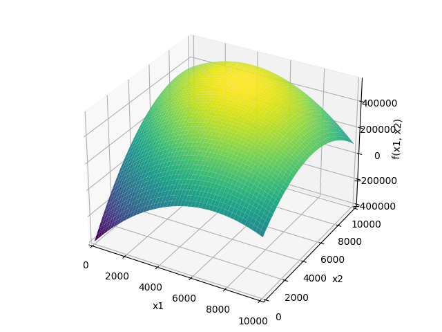
# 是一个曲面
plot3d(fx, (x1, 0, 10000), (x2, 0, 10000))

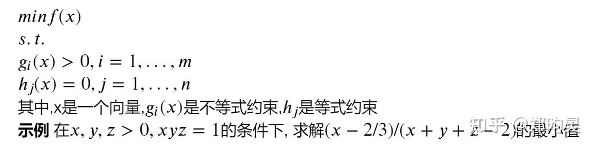
1 求解带有约束的最小化问题

from scipy.optimize import minimize
e = 1e-10
fun = lambda x:(x[0] - 0.667) / (x[0] + x[1] + x[2] - 2) # 目标函数
cons = ({'type':'eq','fun':lambda x:x[0] * x[1] * x[2] - 1}, #约束条件：xyz=1
        {'type':'ineq','fun':lambda x:x[0] - e},             #x,y,z都分别大于0
        {'type':'ineq','fun':lambda x:x[1] - e},
        {'type':'ineq','fun':lambda x:x[2] - e})

x0 = np.array((1.0,1.0,1.0)) #设置xyz的初始值
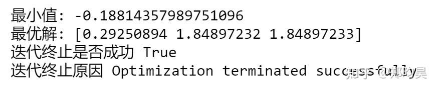
res = minimize(fun,x0,method='SLSQP',constraints=cons)
print("最小值:",res.fun)
print("最优解:",res.x)
print("迭代终止是否成功",res.success)
print("迭代终止原因",res.message)

2 求解不带约束的最小化问题

使用工具：scipy.optimize.minimize

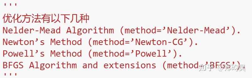
在使用scipy.optimize.minimize求解最小化时，优化器可以选择4种，分别是：

• Nelder-Mead
• Newton-CG
• Powell
• BFGS

BFGS算法的拓展阅读：https://machinelearningmastery.com/bfgs-optimization-in-python/

Nelder-Mean算法的拓展阅读：https://machinelearningmastery.com

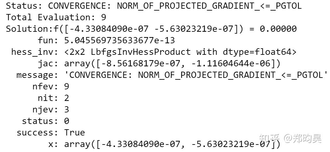
from scipy.optimize import minimize
from numpy.random import rand

# 两个未知数
def objective(x):
    return x[0]**2.0 + x[1]**2

r_min,r_max = -5.0,5.0

# 生成随机初始值
pt = r_min + rand(2) * (r_max - r_min)

result = minimize(objective,pt,method='L-BFGS-B')

print("Status: %s" %result['message'])
print("Total Evaluation: %d" %result['nfev'])

solution = result['x']
evaluation = objective(solution)
print("Solution:f(%s) = %.5f" %(solution,evaluation))
print(result)

3 求解线性优化问题

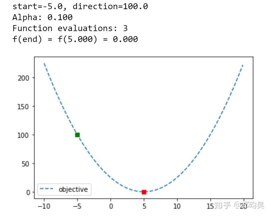
使用工具：scipy.optimize.line_search

对于凸函数寻求线性求解。

from numpy import arange
from scipy.optimize import line_search
from matplotlib import pyplot

# 目标函数
def objective(x):
    return (-5.0 + x)**2.0

# 目标函数的导函数
def gradient(x):
    return 2.0 * (-5.0 + x)

# 定义开始点
point = -5.0
# 定义移动方位
direction = 100.0
# 打印初始条件
print('start=%.1f, direction=%.1f' % (point, direction))

# 执行线性优化函数,传入目标函数objective,导函数gradident,初始点point,移动方位direction
result = line_search(objective, gradient, point, direction)

# 得到结果,求解出alpha，前进的最优幅度
alpha = result[0]
print('Alpha: %.3f' % alpha)
print('Function evaluations: %d' % result[1])

# define objective function minima
end = point + alpha * direction
# evaluate objective function minima
print('f(end) = f(%.3f) = %.3f' % (end, objective(end)))


# define range
r_min, r_max = -10.0, 20.0
# prepare inputs
inputs = arange(r_min, r_max, 0.1)
# compute targets
targets = [objective(x) for x in inputs]
# plot inputs vs objective
pyplot.plot(inputs, targets, '--', label='objective')
# plot start and end of the search
pyplot.plot([point], [objective(point)], 's', color='g')
pyplot.plot([end], [objective(end)], 's', color='r')
pyplot.legend()
pyplot.show()

4 求解线性规划问题

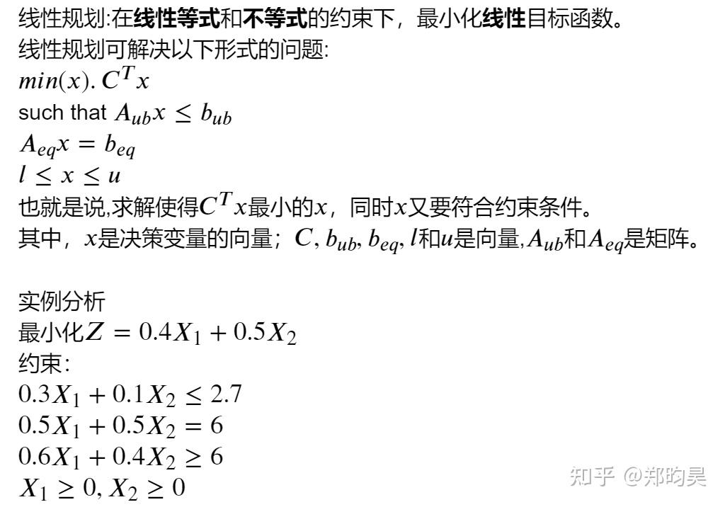
使用工具：scipy.optimize.linprog

import numpy as np
from scipy.optimize import linprog

C = np.array([0.4,0.5])                                # 目标函数的系数 
A_ub = np.array([[0.3,0.1],[-0.6,-0.4]])               # 不等式约束的系数
b_ub = np.array([2.7,-6])                              # 不等式约束的值
A_eq = np.array([[0.5,0.5]])                           # 等式约束的系数
b_eq = np.array([6])                                   # 等式约束的值
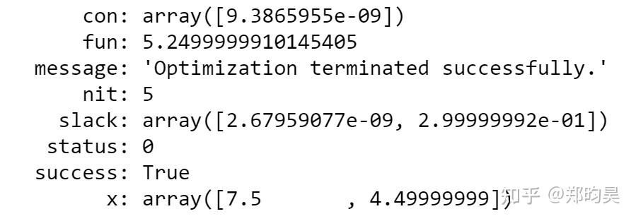
r = linprog(C,A_ub,b_ub,A_eq,b_eq,bounds=((0,None),(0,None)))
print(r)

5 求解全局最优化

求解全局优化有若干种方法，scipy中提供了三种，分别是：

• basinhopping() (盆地跳跃算法)
• differential_evolution() (微分进化算法)
• dual_annealing() (双重模拟退火算法)

5.1 双重模拟退火算法(dual_annealing)

使用工具：scipy.optimize.dual_annealing

Similated Annealing算法的拓展阅读：

https://machinelearningmastery.com/dual-annealing-optimization-with-python/

https://machinelearningmastery.com

# 导入优化包
from scipy.optimize import dual_annealing,basinhopping,differential_evolution
# simulated annealing global optimization for a multimodal objective function


# objective function
def objective(x):
    return (x[0]**2 + x[1] - 11)**2 + (x[0] + x[1]**2 - 7)**2

# 定义x和y的范围
r_min, r_max = -5.0, 5.0
# define the bounds on the search
bounds = [[r_min, r_max], [r_min, r_max]]

# 执行模拟退火算法
# perform the simulated annealing search
result = dual_annealing(objective, bounds)
# summarize the result
print('Status : %s' % result['message'])
print('Total Evaluations: %d' % result['nfev'])
# evaluate solution
solution = result['x']
evaluation = objective(solution)
print('Solution: f(%s) = %.5f' % (solution, evaluation))
print(result)

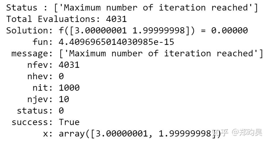
5.2 盆地跳跃算法(basinhopping)

使用工具：scipy.optimize.basinhopping

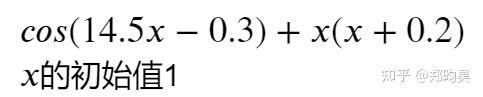
5.2.1 basinhopping求解单目标

from scipy.optimize import basinhopping
# 定义目标函数
func = lambda x:np.cos(14.5 * x - 0.3) + (x + 0.2) * x
# 定义带求解变量初始值
x0 = [1.0]
minimizer_kwargs = {"method":"BFGS"}                 #优化器使用BFGS

ret = basinhopping(func,x0,minimizer_kwargs=minimizer_kwargs,niter=200)
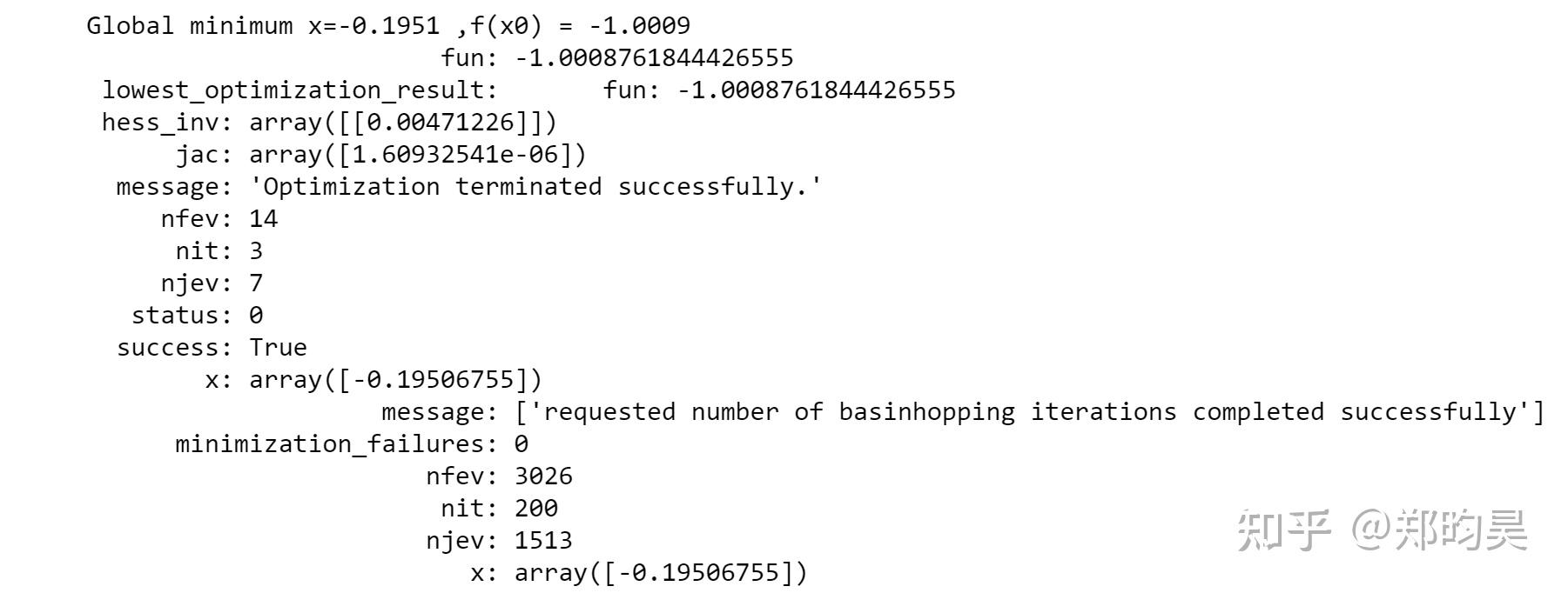
print("Global minimum x=%.4f ,f(x0) = %.4f" %(ret.x,ret.fun))
print(ret)

这里的优化器也可以使用：Nelder-Mead、Powell

5.2.2 basinhopping求解多目标

# simulated annealing global optimization for a multimodal objective function
from scipy.optimize import dual_annealing,basinhopping,differential_evolution

def func2d(x):
    f = np.cos(14.5 * x[0] - 0.3) + (x[1] + 0.2) * x[1] + (x[0] + 0.2) * x[0]
    df = np.zeros(2)
    df[0] = -14.5 * np.sin(14.5 * x[0] - 0.3) + 2. * x[0] + 0.2
    df[1] = 2 * x[1] + 0.2
    return f,df

minimizer_kwargs = {"method":"L-BFGS-B","jac":True}
x0 = [1.0,1.0]
ret = basinhopping(func2d,x0,minimizer_kwargs=minimizer_kwargs,niter=200)
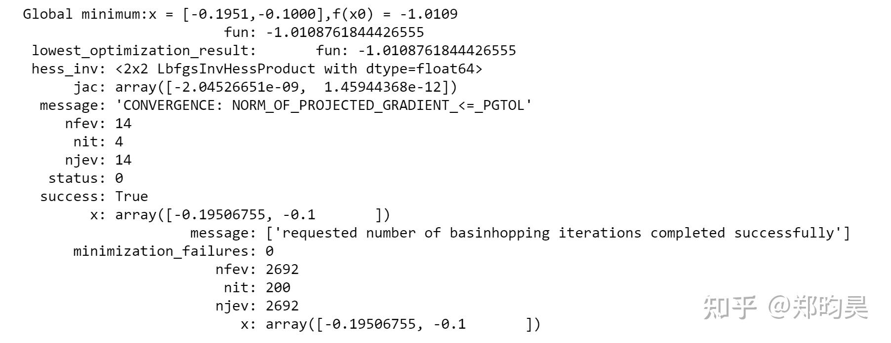
print("Global minimum:x = [%.4f,%.4f],f(x0) = %.4f" %(ret.x[0],ret.x[1],ret.fun))

5.3 微分进化算法(differential_evolution)

使用工具：scipy.optimize.differential_evolution

5.3.1 不带约束

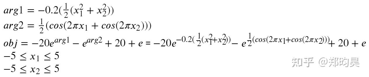
from scipy.optimize import differential_evolution
import numpy as np

# 定义目标函数
def ackley(x):
    arg1 = -0.2 * np.sqrt(0.5 * (x[0] ** 2 + x[1] ** 2))
    arg2 = 0.5 * (np.cos(2. * np.pi * x[0]) + np.cos(2. * np.pi * x[1]))
    return -20. * np.exp(arg1) - np.exp(arg2) + 20. + np.e
# 定义x和y的范围
bounds = [(-5, 5), (-5, 5)]

# 执行微分进化算法
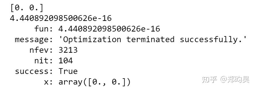
result = differential_evolution(ackley, bounds)
result.x, result.fun

5.3.2 带约束

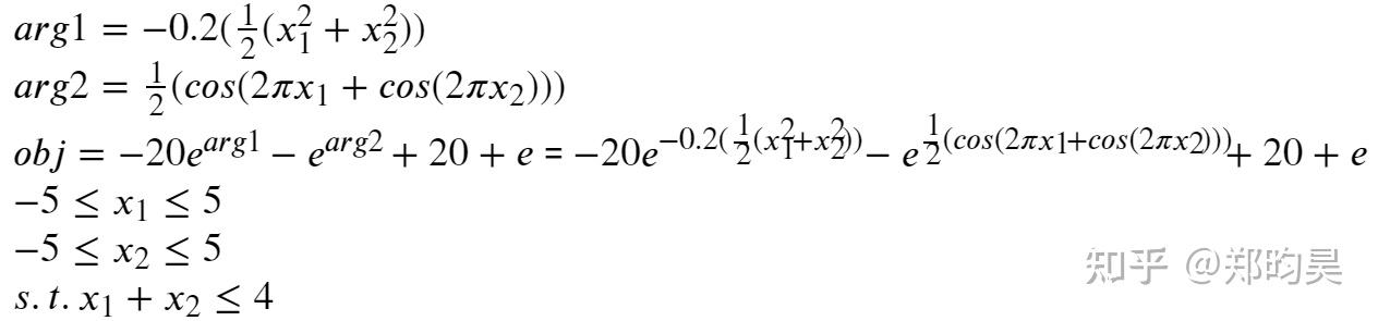
一个约束

from scipy.optimize import differential_evolution,NonlinearConstraint
import numpy as np

# 定义目标函数
def ackley(x):
    arg1 = -0.2 * np.sqrt(0.5 * (x[0] ** 2 + x[1] ** 2))
    arg2 = 0.5 * (np.cos(2. * np.pi * x[0]) + np.cos(2. * np.pi * x[1]))
    return -20. * np.exp(arg1) - np.exp(arg2) + 20. + np.e
bounds = [(-5, 5), (-5, 5)]

# 定义约束条件
def constr_f(x):
    return np.array(x[0] + 2*x[1])

# 实例约束条件
# x1+x2<=4
nlc = NonlinearConstraint(constr_f,-np.inf,4)

result = differential_evolution(ackley, bounds,constraints=(nlc))
print(result.x), print(result.fun)
print(result)

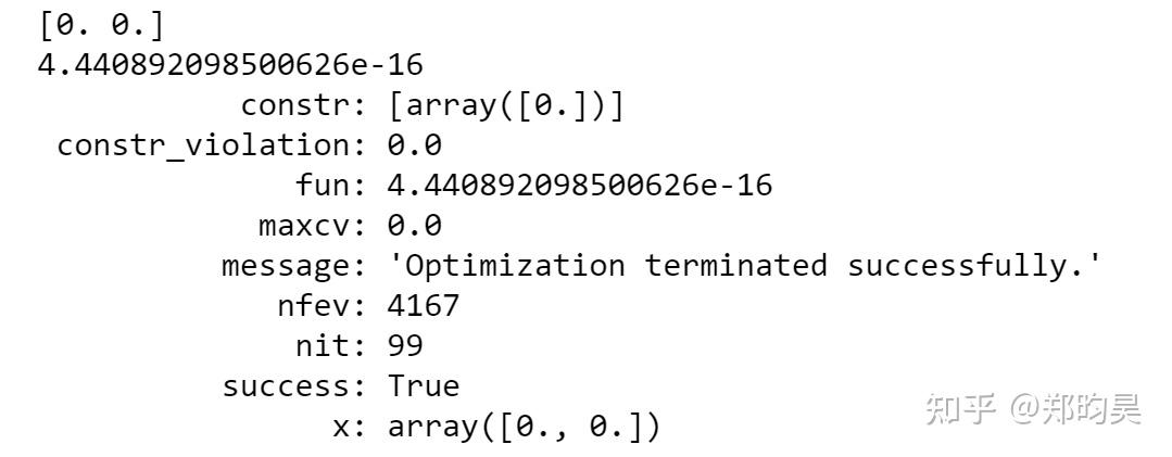
两个约束

from scipy.optimize import differential_evolution
import numpy as np
def ackley(x):
    arg1 = -0.2 * np.sqrt(0.5 * (x[0] ** 2 + x[1] ** 2))
    arg2 = 0.5 * (np.cos(2. * np.pi * x[0]) + np.cos(2. * np.pi * x[1]))
    return -20. * np.exp(arg1) - np.exp(arg2) + 20. + np.e
bounds = [(-5, 5), (-5, 5)]

# 设置两个约束条件
def constr_f1(x):
    return np.array(x[0]*x[1])
def constr_f2(x):
    return np.array(x[0] + 2*x[1])

# x1+x2<=4
nlc1 = NonlinearConstraint(constr_f1,-np.inf,4)
nlc2 = NonlinearConstraint(constr_f2,-np.inf,4)

result = differential_evolution(ackley, bounds,constraints=(nlc1,nlc2))
print(result.x), print(result.fun)
print(result)

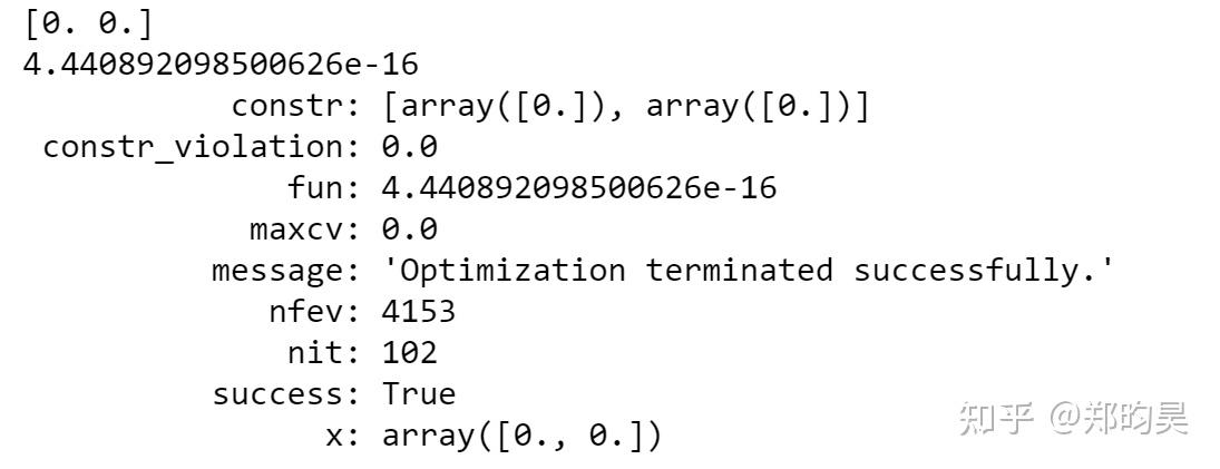
6 求解二次规划

使用工具：cvxopt.matrix、cvxopt.solvers

6.1 例子1

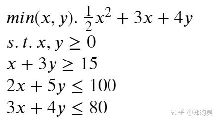
from cvxopt import matrix
from cvxopt import solvers

P = matrix([[1.0,0.0],[0.0,0.0]])                   # P二次型系数矩阵
q = matrix([3.0,4.0])                               # 一次项的系数矩阵
G = matrix([[-1.0,0.0,-1.0,2.0,3.0],[0.0,-1.0,-3.0,5.0,4.0]])  # 约束条件系数矩阵
h = matrix([0.0,0.0,-15.0,100.0,80.0])                         # 约束条件常数矩阵

# 求解二次规划
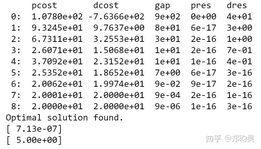
sol = solvers.qp(P,q,G,h)

sol['x']
sol['primal objective']

print(sol['x'])

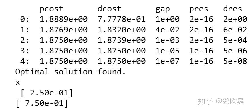
6.2 例子2

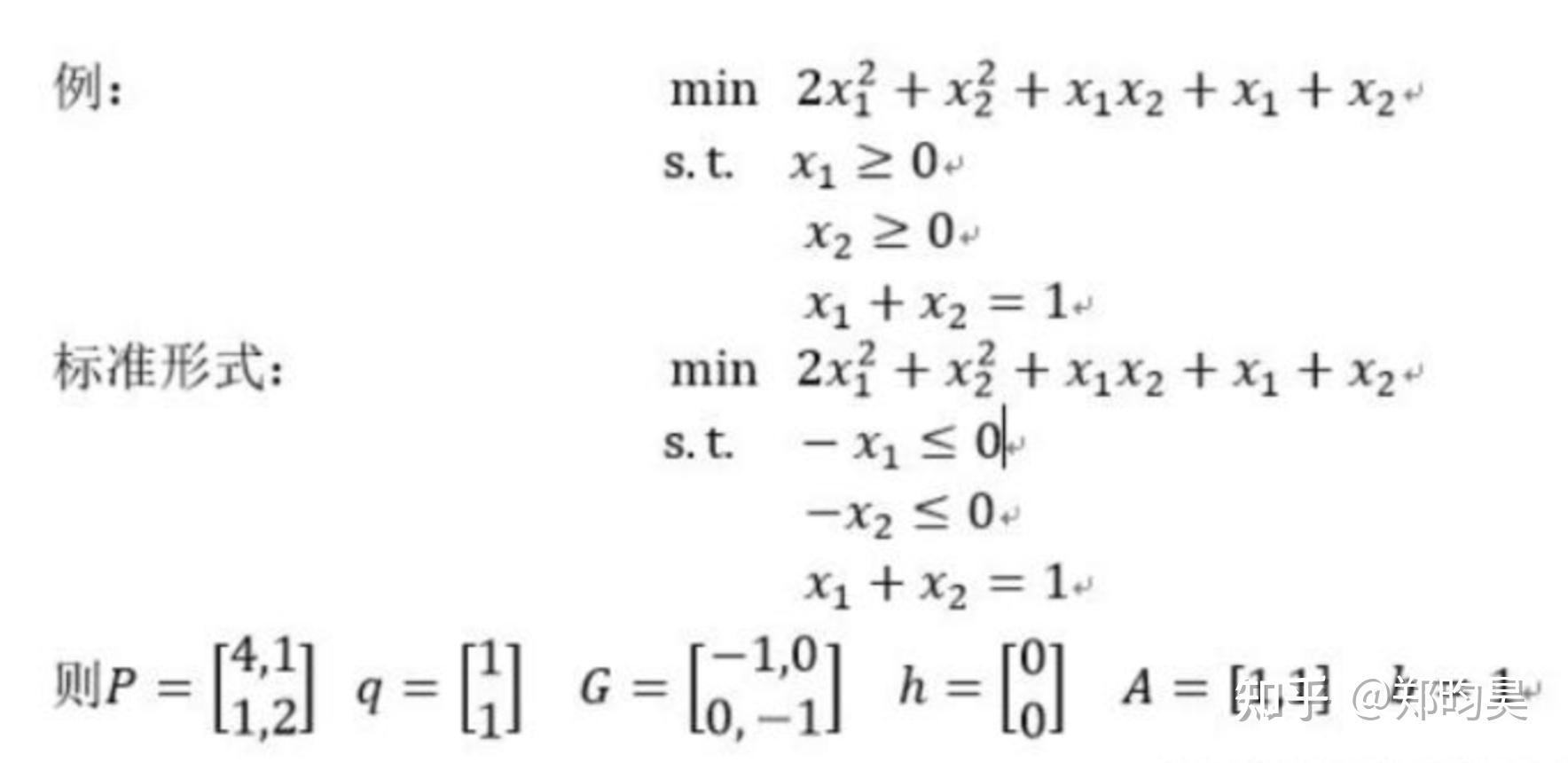
import pprint
from cvxopt import matrix, solvers
P = matrix([[4.0,1.0],[1.0,2.0]])           # 二次型系数矩阵
q = matrix([1.0,1.0])                       # 一次项系数矩阵
G = matrix([[-1.0,0.0],[0.0,-1.0]])         # 不等式约束系数矩阵
h = matrix([0.0,0.0])                       # 不等式约束常数矩阵
#A = matrix([1.0,1.0],(1,2))#原型为cvxopt.matrix(array,dims)，等价于A = matrix([[1.0],[1.0]]）
A = matrix([[1.0],[1.0]])                   # 等式约束常数矩阵
b = matrix([1.0])                           # 等式约束常数值
result = solvers.qp(P,q,G,h,A,b)
 
print('x\n',result['x'])

参考资料

[1] Python–使用scipy求解带约束的最优化问题_爱吃汉堡薯条的博客-CSDN博客

[2] 使用scipy.optimize.linprog求解线性规划问题_weixin_43638511的博客-CSDN博客

[3] A Gentle Introduction to the BFGS Optimization Algorithm - Machine Learning Mastery

[4] https://machinelearningmastery.com/dual-annealing-optimization-with-python/

[5] https://machinelearningmastery.com/simulated-annealing-from-scratch-in-python/

mastery.com/bfgs-optimization-in-python/)

[4] https://machinelearningmastery.com/dual-annealing-optimization-with-python/

[5] https://machinelearningmastery.com/simulated-annealing-from-scratch-in-python/

[6] https://machinelearningmastery.com