原理

最小二乘法进行线性拟合分为训练过程和预测过程

训练过程分为如下3步：
       ①导入训练数据集，得到特征值feature（即X）和标签label（即Y）
       ②利用最小二乘法进行训练，根据公式得到W
       ③将W保存

预测过程分为如下4步：
       ①导入测试数据集，得到测试集的特征值feature
       ②导入W
       ③根据公式得预测值predict
       ④将预测值保存

权重向量

 w = np.matmul(np.matmul(feature.T, feature).I, np.matmul(feature.T, label))

预测结果

 即：

predict = np.matmul(testData, w.T)

源数据(200行)

最小二乘法完整代码

训练过程

import numpy as np

# 导入训练数据集data.txt
def load_data(file_name):
    '''导入数据
    input:  file_path(string):训练数据
    output: feature(mat):特征
            label(mat):标签
    '''

    f = open(file_name)

    feature = []
    label = []

    for line in f.readlines():
        feature_tmp = []
        lines = line.strip().split("\t")
        # print(lines)
        feature_tmp.append(1)  # x0

        for i in range(len(lines) - 1):
            feature_tmp.append(float(lines[i]))
        feature.append(feature_tmp)
        label.append(float(lines[-1]))

    f.close()
    #   print(np.mat(feature))
    #   print(np.mat(label).T)
    #   矩阵化
    return np.mat(feature), np.mat(label).T  # 至此导入数据已经完成


# 导入数据后，用最小二乘法对参数进行训练
def least_square(feature, label):
    '''
    input: feature,label
    output: w
    '''
    #   print(feature.shape)
    #   print(label.shape)
    #   print(label)
    #   叉乘
    w = np.matmul(np.matmul(feature.T, feature).I, np.matmul(feature.T, label))
    #   print(w.shape)
    return w.T

# 训练完成后，将最终的线性回归模型参数保存在文件"weights.txt"
def save_model(file_name, w):
    '''保存最终的模型
    input：file_name(string):要保存的文件的名称
            w(mat):训练好的线性回归模型
    '''
    f_result = open(file_name, "w")  # 以写的模式打开

    m, n = np.shape(w)  # m表示行数，n表示列数
    #    print(m,n)
    for i in range(m):
        w_tmp = []
        for j in range(n):
            w_tmp.append(str(w[i, j]))
        f_result.write("\t".join(w_tmp) + "\n")

    f_result.close()

# 训练过程的主函数
if __name__ == "__main__":
    # 1、导入数据集
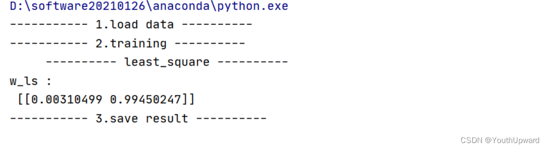
    print("----------- 1.load data ----------")
    # 用feature,label接收两个返回值
    feature, label = load_data(r"C:\Users\YouthUpward\Desktop\机器学习\实验2 线性回归\data.txt")

    # 2、最小二乘法求解
    print("----------- 2.training ----------")
    print("\t ---------- least_square ----------")
    w_ls = least_square(feature, label)
    print("w_ls :\n",w_ls)

    # 3、保存最终的结果
    print("----------- 3.save result ----------")
    save_model(r"C:\Users\YouthUpward\Desktop\机器学习\实验2 线性回归\weights.txt", w_ls)

预测过程

import numpy as np

# 导入数据
def load_data(file_name):
    '''导入数据
    input:  file_path(string):测试数据
    output: feature 转化成矩阵形式的特征值
    '''
    f = open(file_name)

    feature = []

    for line in f.readlines():
        feature_tmp = []
        lines = line.strip().split("\t")
        # print(lines)
        feature_tmp.append(1)  # x0

        for i in range(len(lines)):
            feature_tmp.append(float(lines[i]))
        feature.append(feature_tmp)

    f.close()
    return np.mat(feature)  # 至此导入数据已经完成


# 导入线性回归模型
def load_model(file_name):

    f = open(file_name)  # 读入文件
    w = []
    for line in f.readlines():  # 对于文件的每一行
        w_tmp = []
        lines = line.strip().split("\t")
        for i in range(len(lines)):
            w_tmp.append(float(lines[i]))
        w.append(w_tmp)
#    print("w = ", w)
    f.close()
    return np.mat(w)


# 得到预测结果，X值与w叉乘
def get_prediction(testData, w):
#    print(testData.shape)
#    print(w.T.shape)
    predict = np.matmul(testData, w.T)

    return np.mat(predict)


# 保存预测结果,将Y值保存在“predict_result.txt”文件中
def save_predict(file_name, predict):
    f = open(file_name, "w")  # 写入文件

    m, n = np.shape(predict)  # m表示行数，n表示列数

    for i in range(m):
        predict_tmp = []
        for j in range(n):
            predict_tmp.append(str(predict[i, j]))
        f.write("\t".join(predict_tmp) + "\n")

    f.close()


# 测试过程的主函数
if __name__ == "__main__":
    # 1、导入测试数据
    testData = load_data(r"C:\Users\YouthUpward\Desktop\机器学习\实验2 线性回归\data_test.txt")

    # 2、导入线性回归模型
    w = load_model(r"C:\Users\YouthUpward\Desktop\机器学习\实验2 线性回归\weights.txt")

    # 3、得到预测结果
    predict = get_prediction(testData, w)
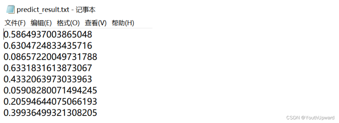
    print(predict)
    
    # 4、保存最终的结果
    save_predict(r"C:\Users\YouthUpward\Desktop\机器学习\实验2 线性回归\predict_result.txt", predict)

最小二乘法图的绘制

import matplotlib.pyplot as plt
import numpy as np

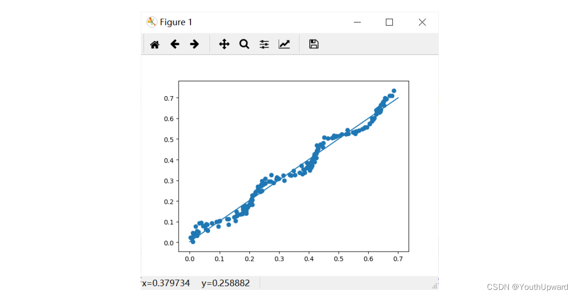
#首先要绘制散点图，其次要绘制一次函数
f = open(r"C:\Users\YouthUpward\Desktop\机器学习\实验2 线性回归\data.txt")
feature = []
label = []
for line in f.readlines():
    lines = line.strip().split("\t")
    feature.append(float(lines[0]))
    label.append(float(lines[1]))
#print(feature)
#print(label)
f.close()


f = open(r"C:\Users\YouthUpward\Desktop\机器学习\实验2 线性回归\weights.txt")
w = []
for line in f.readlines():
    lines = line.strip().split("\t")
    w.append(lines[0])
    w.append(lines[1])
f.close()

plt.figure()
plt.scatter(feature,label)  #散点图


x = np.arange(0,0.8,0.1)
y = []
for i in range(len(x)):
    y.append(float(w[0]) + float(w[1]) * x[i])

plt.plot(x,y)
plt.show()