一、单变量线性回归：

导入相关库：

import numpy as np
import pandas as pd
import matplotlib.pyplot as plt

 读取csv数据文件并查看数据集的前五行

f = pd.read_csv('work/ex1data1.txt', names=['Population', 'Profit'])
f.head()

 

 可视化该数据集

f.plot(kind='scatter', x='Population', y='Profit')
plt.show()

 

损失函数计算：

def computeCost(X, Y, theta):
    cost = np.power((X * theta.T - Y), 2)
    return np.sum(cost) / (2 * len(X))

在f的第一列插入常数1

f.insert(0, 'ones', 1)
cols = f.shape[1]
f

 

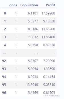
 定义梯度更新函数：

def gradientUpdate(epoch, alpha, X, Y, theta):
    theta1 = np.matrix([0, 0])
    cost = []
    for i in range(epoch):
        theta1 = theta
        theta = theta1 - (alpha / len(X)) * (X * theta.T - Y).T * X
        cost1 = computeCost(X, Y, theta)
        cost.append(cost1)
    return theta, cost

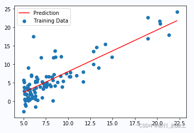
画图，观察决策边界：

x = np.linspace(f.Population.min(), f.Population.max(), 100)
y = final_theta[0,0] + (final_theta[0,1]*x)

fig, ax = plt.subplots(figsize=(6,4))
ax.plot(x, y, 'r', label='Prediction')
ax.scatter(f.Population, f.Profit, label='Training Data')
ax.legend(loc=2)
plt.show()

fig, ax = plt.subplots(figsize=(8,4))
ax.plot(np.arange(epoch), cost, 'r')
ax.set_xlabel('Iterations')
ax.set_ylabel('Cost')
ax.set_title('Error vs. Training Epoch')
plt.show()

二、多变量线性回归：

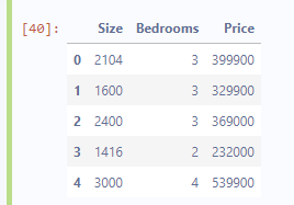
 读取第二个作业文件：

f2 = pd.read_csv('work/ex1data2.txt', names=['Size', 'Bedrooms', 'Price'])
f2.head()

 

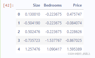
 特征缩放：

f2 = (f2 - f2.mean()) / f2.std()
f2.head()

绘制并观察损失曲线：

fig, ax = plt.subplots(figsize=(12,8))
ax.plot(np.arange(epoch), cost, 'r')
ax.set_xlabel('Iterations')
ax.set_ylabel('Cost')
ax.set_title('Error')
plt.show()

三、正规方程：

 定义函数：

def normalEqn(X, y):
    theta = np.linalg.inv(X.T * X) * X.T * y
    return theta
final_theta2 = normalEqn(X, Y)
x = np.linspace(f.Population.min(), f.Population.max(), 100)
y = final_theta2[0,0] + (final_theta2[1,0]*x)

fig, ax = plt.subplots(figsize=(6,4))
ax.plot(x, y, 'r', label='Prediction')
ax.scatter(f.Population, f.Profit, label='Training Data')
ax.legend(loc=2)
plt.show()

 发现效果也不错