---

一. 生成数据集

我们使用线性模型参数 w=[2,−3.4]⊤ 、 b=4.2 和噪声项 ϵ 生成数据集及其标签：

$$\mathbf{y}=\mathbf{X}\mathbf{w}+b+ϵ$$
在这里我们认为标准假设成立，即 ϵ 服从均值为0的正态分布。 为了简化问题，我们将标准差设为0.01。下面的代码生成合成数据集。

def synthetic_data(w, b, num_examples):  #@save
    """生成 y = Xw + b + 噪声。"""
    X = torch.normal(0, 1, (num_examples, len(w)))
    y = torch.matmul(X, w) + b
    y += torch.normal(0, 0.01, y.shape)
    return X, y.reshape((-1, 1))

true_w = torch.tensor([2, -3.4])
true_b = 4.2
features, labels = synthetic_data(true_w, true_b, 1000)

features中的每一行都包含一个二维数据样本，labels中的每一行都包含一维标签值（一个标量）。

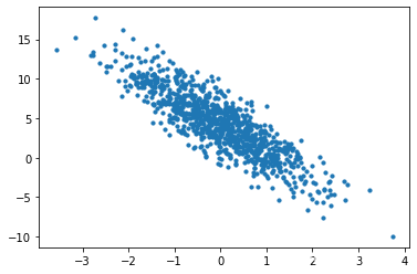
通过生成第二个特征features[:, 1]和labels的散点图，可以直观地观察到两者之间的线性关系。

xx = np.zeros(1000)
yy = np.zeros(1000)
for i in range(1000) :
    a = features[i]
    #xx[i] = float(a[0])
    xx[i] = float(a[1])
    yy[i] = labels[i]
plt.scatter(xx, yy, 10)

二. 线性回归实现

1. 批量读取

定义一个data_iter函数， 该函数接收批量大小、特征矩阵和标签向量作为输入，生成大小为batch_size的小批量。每个小批量包含一组特征和标签。

def data_iter(batch_size, features, labels):
    num_examples = len(features)
    indices = list(range(num_examples))
    # 这些样本是随机读取的，没有特定的顺序
    random.shuffle(indices)
    for i in range(0, num_examples, batch_size):
        batch_indices = torch.tensor(
            indices[i: min(i + batch_size, num_examples)])
        yield features[batch_indices], labels[batch_indices]

读取第一个小批量数据样本并打印。每个批量的特征维度说明了批量大小和输入特征数。

batch_size = 10

for X, y in data_iter(batch_size, features, labels):
    print(X, '\n', y)
    break

tensor([[-0.5844,  0.0211],
        [-0.8453, -0.1036],
        [-0.7383,  0.1296],
        [ 1.1084,  0.9297],
        [-1.4047, -1.0691],
        [ 0.8032,  1.9856],
        [ 0.2277,  0.9269],
        [-0.1643, -1.6299],
        [-1.0487,  0.3702],
        [ 0.9363, -1.5222]]) 
 tensor([[ 2.9408],
        [ 2.8535],
        [ 2.2959],
        [ 3.2462],
        [ 5.0288],
        [-0.9618],
        [ 1.4876],
        [ 9.4235],
        [ 0.8321],
        [11.2567]])

2.初始化模型参数

w = torch.normal(0, 0.01, size=(2,1), requires_grad=True)
b = torch.zeros(1, requires_grad=True)

3.定义模型，损失函数，优化算法

def linreg(X, w, b):  
    """线性回归模型。"""
    return torch.matmul(X, w) + b

def squared_loss(y_hat, y):  #@save
    """均方损失。"""
    return (y_hat - y.reshape(y_hat.shape)) ** 2 / 2

def sgd(params, lr, batch_size):  #@save
    """小批量随机梯度下降。"""
    with torch.no_grad():
        for param in params:
            param -= lr * param.grad / batch_size
            param.grad.zero_()

4. 训练

lr = 0.03
num_epochs = 3
net = linreg
loss = squared_loss

for epoch in range(num_epochs):
    for X, y in data_iter(batch_size, features, labels):
        l = loss(net(X, w, b), y)  # `X`和`y`的小批量损失
        # 因为`l`形状是(`batch_size`, 1)，而不是一个标量。`l`中的所有元素被加到一起，
        # 并以此计算关于[`w`, `b`]的梯度
        l.sum().backward()
        sgd([w, b], lr, batch_size)  # 使用参数的梯度更新参数
    with torch.no_grad():
        train_l = loss(net(features, w, b), labels)
        print(f'epoch {epoch + 1}, loss {float(train_l.mean()):f}')

epoch 1, loss 0.029955
epoch 2, loss 0.000098
epoch 3, loss 0.000048

print(f'w的估计误差: {true_w - w.reshape(true_w.shape)}')
print(f'b的估计误差: {true_b - b}')

w的估计误差: tensor([0.0010, 0.0004], grad_fn=<SubBackward0>)
b的估计误差: tensor([2.0504e-05], grad_fn=<RsubBackward1>)

三. 线性回归的框架实现

1.读取数据集

def load_array(data_arrays, batch_size, is_train=True):  
    """构造一个PyTorch数据迭代器。"""
    dataset = data.TensorDataset(*data_arrays)#from torch.utils import data
    return data.DataLoader(dataset, batch_size, shuffle=is_train)

batch_size = 10
data_iter = load_array((features, labels), batch_size)

2.定义模型

# `nn` 是神经网络的缩写
from torch import nn

net = nn.Sequential(nn.Linear(2, 1))

3.初始化参数

net[0].weight.data.normal_(0, 0.01)
net[0].bias.data.fill_(0)

4.定义损失函数及优化算法

loss = nn.MSELoss()

trainer = torch.optim.SGD(net.parameters(), lr=0.03)

5.训练

num_epochs = 3
for epoch in range(num_epochs):
    for X, y in data_iter:
        l = loss(net(X) ,y)
        trainer.zero_grad()
        l.backward()
        trainer.step()
    l = loss(net(features), labels)
    print(f'epoch {epoch + 1}, loss {l:f}')

epoch 1, loss 0.000187
epoch 2, loss 0.000096
epoch 3, loss 0.000095

w = net[0].weight.data
print('w的估计误差：', true_w - w.reshape(true_w.shape))
b = net[0].bias.data
print('b的估计误差：', true_b - b)

w的估计误差： tensor([ 0.0010, -0.0002])
b的估计误差： tensor([0.0006])