机器学习实战2之科比篮球生涯得分数据分析
·
import numpy as np
import pandas as pd
import matplotlib.pyplot as plt
导入数据
filename = './data/kobe.csv'
raw = pd.read_csv(filename)
print(raw.shape)
print(raw.head())
(30697, 25)
         action_type combined_shot_type  game_event_id   game_id      lat  \
0          Jump Shot          Jump Shot             10  20000012  33.9723
1          Jump Shot          Jump Shot             12  20000012  34.0443
2          Jump Shot          Jump Shot             35  20000012  33.9093
3          Jump Shot          Jump Shot             43  20000012  33.8693
4  Driving Dunk Shot               Dunk            155  20000012  34.0443

   loc_x  loc_y       lon  minutes_remaining  period   ...          shot_type  \
0    167     72 -118.1028                 10       1   ...     2PT Field Goal
1   -157      0 -118.4268                 10       1   ...     2PT Field Goal
2   -101    135 -118.3708                  7       1   ...     2PT Field Goal
3    138    175 -118.1318                  6       1   ...     2PT Field Goal
4      0      0 -118.2698                  6       2   ...     2PT Field Goal

          shot_zone_area  shot_zone_basic  shot_zone_range     team_id  \
0          Right Side(R)        Mid-Range        16-24 ft.  1610612747
1           Left Side(L)        Mid-Range         8-16 ft.  1610612747
2   Left Side Center(LC)        Mid-Range        16-24 ft.  1610612747
3  Right Side Center(RC)        Mid-Range        16-24 ft.  1610612747
4              Center(C)  Restricted Area  Less Than 8 ft.  1610612747

            team_name   game_date    matchup opponent  shot_id
0  Los Angeles Lakers  2000-10-31  LAL @ POR      POR        1
1  Los Angeles Lakers  2000-10-31  LAL @ POR      POR        2
2  Los Angeles Lakers  2000-10-31  LAL @ POR      POR        3
3  Los Angeles Lakers  2000-10-31  LAL @ POR      POR        4
4  Los Angeles Lakers  2000-10-31  LAL @ POR      POR        5

[5 rows x 25 columns]
#取出得分空值对应的样本,剩余的可以用于测试
kobe = raw[pd.notnull(raw['shot_made_flag'])]
print(kobe.shape)
(25697, 25)
数据可视化处理操作
plt.figure(figsize=(10,10))
alpha = 0.02  #alpha用于指定图像颜色的透明度

plt.subplot(1,2,1)
plt.scatter(kobe.loc_x, kobe.loc_y, color='B', alpha=alpha)
plt.title('loc_x && loc_y')

plt.subplot(1,2,2)
plt.scatter(kobe.lon, kobe.lat, color='G', alpha=alpha)
plt.title('lon && lat')
Text(0.5, 1.0, 'lon && lat')
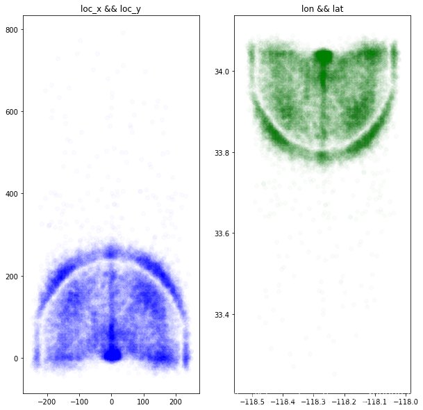
- 投篮坐标和经纬度数据作用一样,只用一个即可,且可以将坐标转换为极坐标
raw['dist'] = np.sqrt(raw['loc_x']**2 + raw['loc_y']**2)

loc_x_zero = raw['loc_x'] == 0
#print (loc_x_zero)
raw['angle'] = np.array([0] * len(raw))
raw['angle'][~loc_x_zero] = np.arctan(
    raw['loc_y'][~loc_x_zero] / raw['loc_x'][~loc_x_zero])
raw['angle'][loc_x_zero] = np.pi / 2
数据预处理,这个很重要
- 将每节剩余分钟数和剩余秒数数据合二为一处理
raw['remaining_time'] = raw['minutes_remaining'] * 60 + raw['seconds_remaining']
- 两个有用的函数,可以分别用来显示一个数据标签中所含有的全部种类,以及每个种类的数量统计
print(kobe.shot_type.unique())
print(kobe.shot_type.value_counts())
['2PT Field Goal' '3PT Field Goal']
2PT Field Goal    20285
3PT Field Goal     5412
Name: shot_type, dtype: int64
- 将pandas中的object类型数据转换为int值,这样机器才能识别
kobe['season'].unique()
array(['2000-01', '2001-02', '2002-03', '2003-04', '2004-05', '2005-06',
       '2006-07', '2007-08', '2008-09', '2009-10', '2010-11', '2011-12',
       '2012-13', '2013-14', '2014-15', '2015-16', '1996-97', '1997-98',
       '1998-99', '1999-00'], dtype=object)
kobe['season'] = kobe['season'].apply(lambda x : int(x.split('-')[1]))
kobe['season'].unique()
array([ 1,  2,  3,  4,  5,  6,  7,  8,  9, 10, 11, 12, 13, 14, 15, 16, 97,
       98, 99,  0], dtype=int64)
print(kobe.team_id.unique())   #无用的数据
print(kobe.team_name.unique())
[1610612747]
['Los Angeles Lakers']
pd.DataFrame({'matchup':kobe.matchup, 'opponent':kobe.opponent})
| matchup | opponent | |
|---|---|---|
| 1 | LAL @ POR | POR |
| 2 | LAL @ POR | POR |
| 3 | LAL @ POR | POR |
| 4 | LAL @ POR | POR |
| 5 | LAL @ POR | POR |
| 6 | LAL @ POR | POR |
| 8 | LAL @ POR | POR |
| 9 | LAL @ POR | POR |
| 10 | LAL @ POR | POR |
| 11 | LAL vs. UTA | UTA |
| 12 | LAL vs. UTA | UTA |
| 13 | LAL vs. UTA | UTA |
| 14 | LAL vs. UTA | UTA |
| 15 | LAL vs. UTA | UTA |
| 17 | LAL vs. UTA | UTA |
| 18 | LAL vs. UTA | UTA |
| 20 | LAL vs. UTA | UTA |
| 21 | LAL vs. UTA | UTA |
| 22 | LAL vs. UTA | UTA |
| 23 | LAL vs. UTA | UTA |
| 24 | LAL vs. UTA | UTA |
| 25 | LAL vs. UTA | UTA |
| 26 | LAL vs. UTA | UTA |
| 27 | LAL vs. UTA | UTA |
| 28 | LAL vs. UTA | UTA |
| 29 | LAL vs. UTA | UTA |
| 30 | LAL vs. UTA | UTA |
| 31 | LAL vs. UTA | UTA |
| 38 | LAL @ VAN | VAN |
| 39 | LAL @ VAN | VAN |
| ... | ... | ... |
| 30661 | LAL @ IND | IND |
| 30662 | LAL @ IND | IND |
| 30663 | LAL @ IND | IND |
| 30665 | LAL @ IND | IND |
| 30666 | LAL @ IND | IND |
| 30667 | LAL @ IND | IND |
| 30669 | LAL @ IND | IND |
| 30670 | LAL vs. IND | IND |
| 30671 | LAL vs. IND | IND |
| 30672 | LAL vs. IND | IND |
| 30673 | LAL vs. IND | IND |
| 30674 | LAL vs. IND | IND |
| 30675 | LAL vs. IND | IND |
| 30676 | LAL vs. IND | IND |
| 30677 | LAL vs. IND | IND |
| 30678 | LAL vs. IND | IND |
| 30679 | LAL vs. IND | IND |
| 30681 | LAL vs. IND | IND |
| 30683 | LAL vs. IND | IND |
| 30684 | LAL vs. IND | IND |
| 30685 | LAL vs. IND | IND |
| 30687 | LAL vs. IND | IND |
| 30688 | LAL vs. IND | IND |
| 30689 | LAL vs. IND | IND |
| 30690 | LAL vs. IND | IND |
| 30691 | LAL vs. IND | IND |
| 30692 | LAL vs. IND | IND |
| 30694 | LAL vs. IND | IND |
| 30695 | LAL vs. IND | IND |
| 30696 | LAL vs. IND | IND |
25697 rows × 2 columns
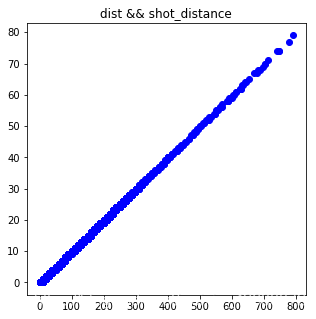
- 强相关数据只选择其中一个即可
plt.figure(figsize=(5,5))
plt.scatter(raw.dist, raw.shot_distance, color='B')
plt.title('dist && shot_distance')
Text(0.5, 1.0, 'dist && shot_distance')
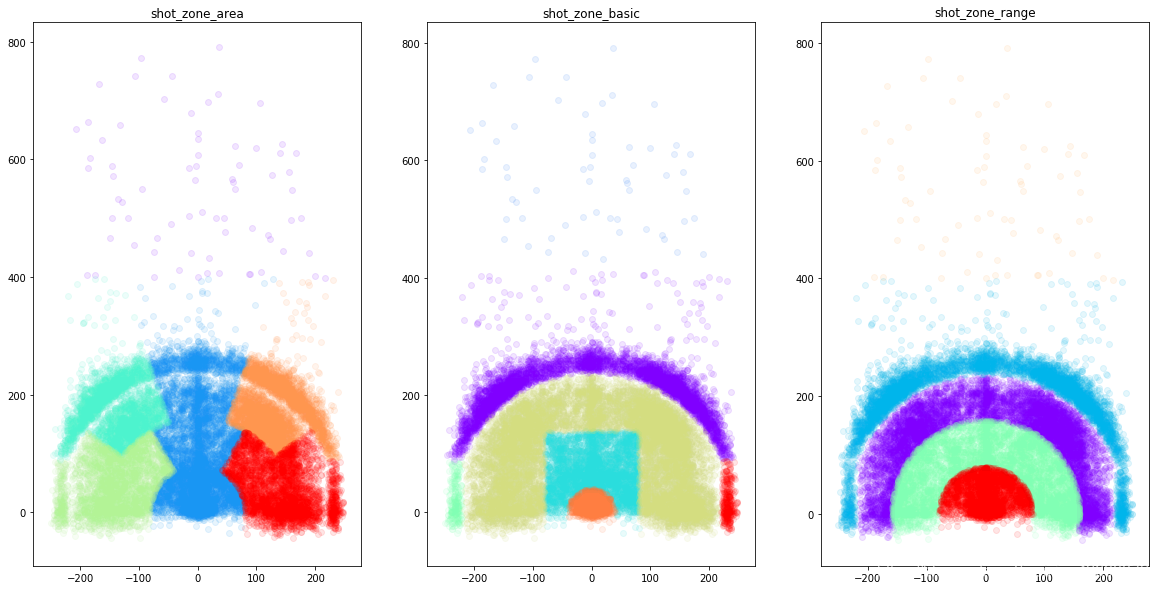
print(kobe['shot_zone_area'].value_counts())
gs = kobe.groupby('shot_zone_area')
print(len(gs))
Center(C)                11289
Right Side Center(RC)     3981
Right Side(R)             3859
Left Side Center(LC)      3364
Left Side(L)              3132
Back Court(BC)              72
Name: shot_zone_area, dtype: int64
6
import matplotlib.cm as cm
plt.figure(figsize=(20,10))

def scatter_plot_by_category(feat):
    alpha = 0.1
    gs = kobe.groupby(feat)
    cs = cm.rainbow(np.linspace(0, 1, len(gs)))
    for g, c in zip(gs, cs):
        plt.scatter(g[1].loc_x, g[1].loc_y, color=c, alpha=alpha)

# shot_zone_area
plt.subplot(131)
scatter_plot_by_category('shot_zone_area')
plt.title('shot_zone_area')

# shot_zone_basic
plt.subplot(132)
scatter_plot_by_category('shot_zone_basic')
plt.title('shot_zone_basic')

# shot_zone_range
plt.subplot(133)
scatter_plot_by_category('shot_zone_range')
plt.title('shot_zone_range')
Text(0.5, 1.0, 'shot_zone_range')
- 丢弃一些无用的数据
drops = ['shot_id', 'team_id', 'team_name', 'shot_zone_area', 'shot_zone_range', 'shot_zone_basic', \
         'matchup', 'lon', 'lat', 'seconds_remaining', 'minutes_remaining', \
         'shot_distance', 'loc_x', 'loc_y', 'game_event_id', 'game_id', 'game_date']
for drop in drops:
    raw = raw.drop(drop, 1)
print (raw['combined_shot_type'].value_counts())
pd.get_dummies(raw['combined_shot_type'], prefix='combined_shot_type')[0:2]
Jump Shot    23485
Layup         5448
Dunk          1286
Tip Shot       184
Hook Shot      153
Bank Shot      141
Name: combined_shot_type, dtype: int64
| combined_shot_type_Bank Shot | combined_shot_type_Dunk | combined_shot_type_Hook Shot | combined_shot_type_Jump Shot | combined_shot_type_Layup | combined_shot_type_Tip Shot | |
|---|---|---|---|---|---|---|
| 0 | 0 | 0 | 0 | 1 | 0 | 0 |
| 1 | 0 | 0 | 0 | 1 | 0 | 0 |
categorical_vars = ['action_type', 'combined_shot_type', 'shot_type', 'opponent', 'period', 'season']
for var in categorical_vars:
    raw = pd.concat([raw, pd.get_dummies(raw[var], prefix=var)], 1)
    raw = raw.drop(var, 1)
建立模型
train_kobe = raw[pd.notnull(raw['shot_made_flag'])]
train_label = train_kobe['shot_made_flag']
train_kobe = train_kobe.drop('shot_made_flag', 1)
test_kobe = raw[pd.isnull(raw['shot_made_flag'])]
test_kobe = test_kobe.drop('shot_made_flag', 1)
from sklearn.ensemble import RandomForestRegressor
from sklearn.metrics import confusion_matrix,log_loss
import time
range_m = np.logspace(0,2,num=5).astype(int)
range_m
array([ 1, 3, 10, 31, 100])
# find the best n_estimators for RandomForestClassifier
from sklearn.ensemble import RandomForestClassifier
from sklearn.model_selection import KFold

print('Finding best n_estimators for RandomForestClassifier...')
min_score = 100000
best_n = 0
scores_n = []
range_n = np.logspace(1, 2, num=8).astype(int)
for n in range_n:
    print("the number of trees : {0}".format(n))
    t1 = time.time()

    rfc_score = 0.
    rfc = RandomForestClassifier(n_estimators=n)
    kf = KFold(n_splits=5, shuffle=True,  random_state=40).split(train_kobe)
    for train_k, test_k in kf:
        rfc.fit(train_kobe.iloc[train_k], train_label.iloc[train_k])
        #rfc_score += rfc.score(train.iloc[test_k], train_y.iloc[test_k])/10
        pred = rfc.predict(train_kobe.iloc[test_k])
        rfc_score += log_loss(train_label.iloc[test_k], pred) / 10
    scores_n.append(rfc_score)
    if rfc_score < min_score:
        min_score = rfc_score
        best_n = n

    t2 = time.time()
    print('Done processing {0} trees ({1:.3f}sec)'.format(n, t2 - t1))
print(best_n, min_score)

# find best max_depth for RandomForestClassifier
print('Finding best max_depth for RandomForestClassifier...')
min_score = 100000
best_m = 0
scores_m = []
range_m = np.logspace(0, 2,num=8).astype(int)
for m in range_m:
    print("the max depth : {0}".format(m))
    t1 = time.time()

    rfc_score = 0.
    rfc = RandomForestClassifier(max_depth=m, n_estimators=best_n)
    kf = KFold(n_splits=5, shuffle=True,  random_state=40).split(train_kobe)
    for train_k, test_k in kf:
        rfc.fit(train_kobe.iloc[train_k], train_label.iloc[train_k])
        #rfc_score += rfc.score(train.iloc[test_k], train_y.iloc[test_k])/10
        pred = rfc.predict(train_kobe.iloc[test_k])
        rfc_score += log_loss(train_label.iloc[test_k], pred) / 10
    scores_m.append(rfc_score)
    if rfc_score < min_score:
        min_score = rfc_score
        best_m = m

    t2 = time.time()
    print('Done processing {0} trees ({1:.3f}sec)'.format(m, t2 - t1))
print(best_m, min_score)
Finding best n_estimators for RandomForestClassifier...
the number of trees : 10
Done processing 10 trees (2.832sec)
the number of trees : 13
Done processing 13 trees (3.499sec)
the number of trees : 19
Done processing 19 trees (5.482sec)
the number of trees : 26
Done processing 26 trees (6.886sec)
the number of trees : 37
Done processing 37 trees (10.694sec)
the number of trees : 51
Done processing 51 trees (14.202sec)
the number of trees : 71
Done processing 71 trees (18.946sec)
the number of trees : 100
Done processing 100 trees (25.590sec)
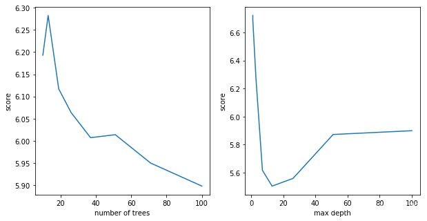
100 5.898521466994053
Finding best max_depth for RandomForestClassifier...
the max depth : 1
Done processing 1 trees (2.554sec)
the max depth : 1
Done processing 1 trees (2.581sec)
the max depth : 3
Done processing 3 trees (3.824sec)
the max depth : 7
Done processing 7 trees (6.487sec)
the max depth : 13
Done processing 13 trees (10.639sec)
the max depth : 26
Done processing 26 trees (18.684sec)
the max depth : 51
Done processing 51 trees (27.133sec)
the max depth : 100
Done processing 100 trees (28.496sec)
13 5.504022676997401
plt.figure(figsize=(10,5))
plt.subplot(121)
plt.plot(range_n, scores_n)
plt.ylabel('score')
plt.xlabel('number of trees')

plt.subplot(122)
plt.plot(range_m, scores_m)
plt.ylabel('score')
plt.xlabel('max depth')
Text(0.5, 0, 'max depth')
model = RandomForestClassifier(n_estimators=best_n, max_depth=best_m)
model.fit(train_kobe, train_label)

北京人形旗下天工造物具身智能开源社区,聚焦具身天工与慧思开物两大平台
更多推荐
 3
3 0
0- 0


 已为社区贡献1条内容

所有评论(0)