本篇博客将按照机器学习简介中机器学习建模步骤，结合宝可梦（神奇宝贝）具体数据进行案例分析。

---

目录

---

Objective

通过训练宝可梦属性的历史数据构建回归模型，输入宝可梦进化前的属性数据，预测宝可梦进化后的Combat Power (CP)。

<script type="math/tex" id="MathJax-Element-48">\quad</script>

step1：Model

假设进化前的 xcp x c p <script type="math/tex" id="MathJax-Element-49">x_{cp}</script>与进化后的 xcp x c p <script type="math/tex" id="MathJax-Element-50">x_{cp}</script>的（即 y y <script type="math/tex" id="MathJax-Element-51">y</script>）存在关系f1,f2…fn,(fi=bi+wixcp,i=1,2…n)$f_1,f_2\dots f_n,(f_i=b_i+w_i{x}_{cp},i=1,2\dots n)$<script type="math/tex" id="MathJax-Element-52">f_1,f_2\dots f_n,(f_i=b_i+w_ix_{cp},i=1,2\dots n)</script>

<script type="math/tex" id="MathJax-Element-53">\quad</script>

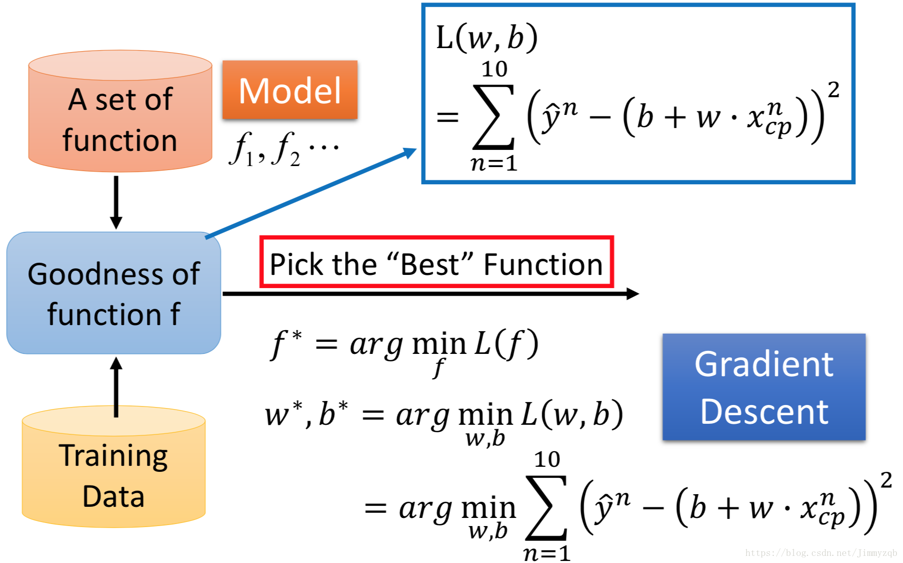
step2：Goodness of Function

xicp x c p i <script type="math/tex" id="MathJax-Element-80">x^i_{cp}</script>表示第 i i <script type="math/tex" id="MathJax-Element-81">i</script>个观测（进化前的CP），ŷ i${\hat{y}}^i$<script type="math/tex" id="MathJax-Element-82">\hat{y}^i</script>表示第 i i <script type="math/tex" id="MathJax-Element-83">i</script>个观测的真实值（进化后的CP），现在捕捉10只宝可梦，记录这10只宝可梦进化前和进化后的CP（xicp,ŷ i,i=1,2…10$x_{cp}^i,{\hat{y}}^i,i=1,2\dots 10$<script type="math/tex" id="MathJax-Element-84">x_{cp}^i,\hat{y}^i,i=1,2\dots10</script>），在这一案例中 L(w,b)=∑10n=1(ŷ n−(b+wxncp))2 L ( w , b ) = ∑ n = 1 10 ( y ^ n − ( b + w x c p n ) ) 2 <script type="math/tex" id="MathJax-Element-85">L(w,b)=\sum_{n=1}^{10}(\hat{y}^n-(b+wx_{cp}^n))^2</script>。

Loss function L由 w,b w , b <script type="math/tex" id="MathJax-Element-86">w,b</script>控制，可视化如图，冷色调代表低 L L <script type="math/tex" id="MathJax-Element-87">L</script>值，暖色调代表高L$L$<script type="math/tex" id="MathJax-Element-88">L</script>值，

<script type="math/tex" id="MathJax-Element-89">\quad</script>

step3：Best Function

从Step1中的 f1,f2…fn f 1 , f 2 … f n <script type="math/tex" id="MathJax-Element-68">f_1,f_2\dots f_n</script>选择最优函数 f∗ f ∗ <script type="math/tex" id="MathJax-Element-69">f^*</script>， f∗=argminf∈FL(f) f ∗ = a r g m i n f ∈ F L ( f ) <script type="math/tex" id="MathJax-Element-70">f^*=argmin_{f \in F}L(f)</script>，在这一案例中，即 w∗,b∗=argminw,bL(w,b) w ∗ , b ∗ = a r g m i n w , b L ( w , b ) <script type="math/tex" id="MathJax-Element-71">w^*,b^*=argmin_{w,b}L(w,b)</script>

求 L L <script type="math/tex" id="MathJax-Element-72">L</script>函数最小值问题一般用梯度下降法来进行计算，步骤如下：

1. 随机初始化w0,b0$w^0,b^0$<script type="math/tex" id="MathJax-Element-73">w^0,b^0</script>
   • 计算函数 L(w,b) L ( w , b ) <script type="math/tex" id="MathJax-Element-74">L(w,b)</script>在 w0,b0 w 0 , b 0 <script type="math/tex" id="MathJax-Element-75">w^0,b^0</script>处的偏导 dLdw|w=w0,dLdb|b=b0 d L d w | w = w 0 , d L d b | b = b 0 <script type="math/tex" id="MathJax-Element-76">\frac{dL}{dw}|_{w=w^0},\frac{dL}{db}|_{b=b^0}</script>， w1:=w0−ηdLdw|w=w0,b1:=b0−ηdLdb|b=b0, w 1 := w 0 − η d L d w | w = w 0 , b 1 := b 0 − η d L d b | b = b 0 , <script type="math/tex" id="MathJax-Element-77">w^1:=w^0-\eta \frac{dL}{dw}|_{w=w^0},b^1:=b^0-\eta \frac{dL}{db}|_{b=b^0},</script>，其中 η η <script type="math/tex" id="MathJax-Element-78">\eta</script>为学习速率（Learning rate）
   • 重复第二步直到 w,b w , b <script type="math/tex" id="MathJax-Element-79">w,b</script>收敛
     

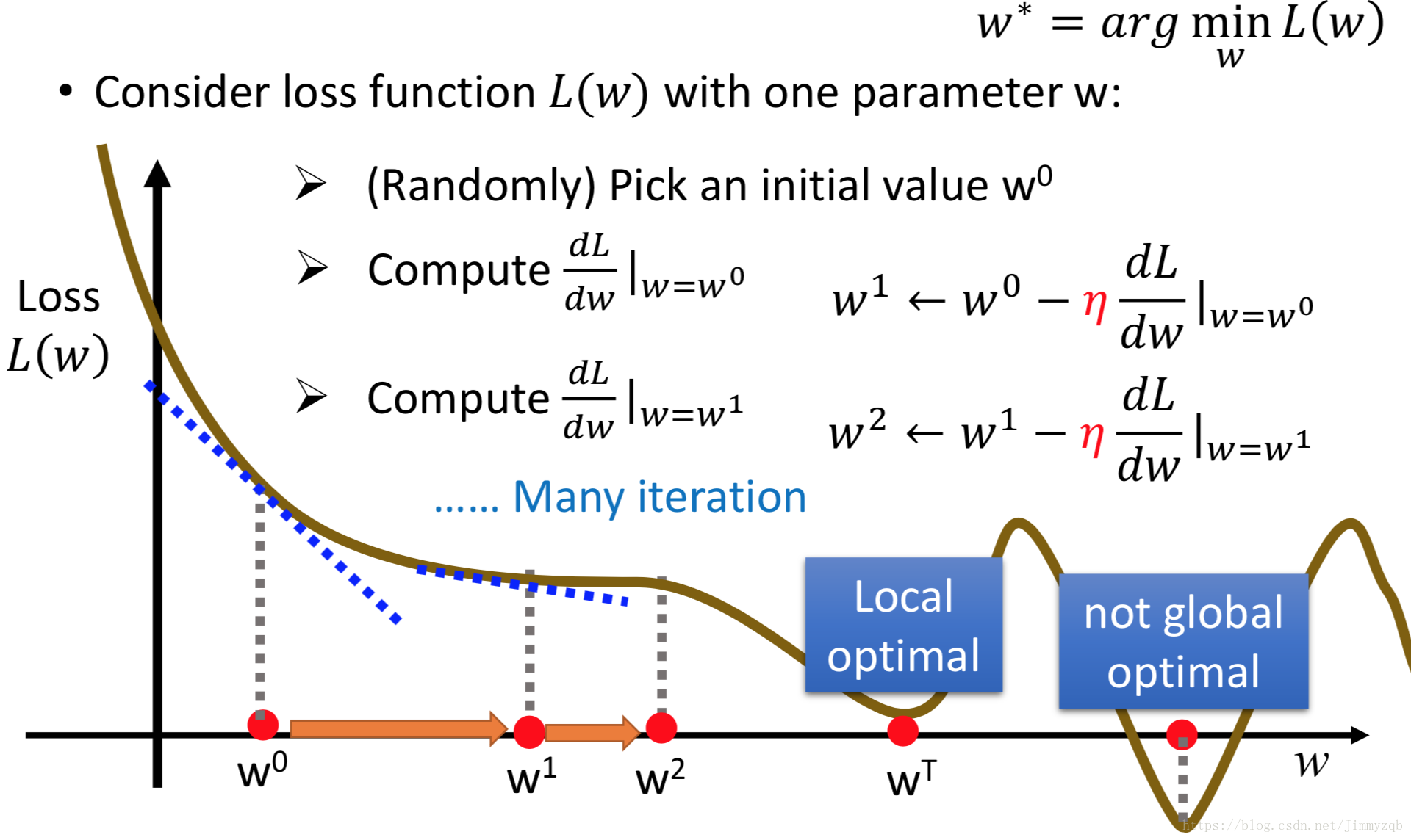
   • 注意：梯度下降方法可能得到的是局部最优，在线性回归模型中，函数是凸的，因此梯度下降得到的最优解即全局最优解

     使用梯度下降算法求解案例最小化问题，
     

     minL(w,b)=min∑n=110(ŷ n−(b+wxncp))2 m i n L ( w , b ) = m i n ∑ n = 1 10 ( y ^ n − ( b + w x c p n ) ) 2
     <script type="math/tex; mode=display" id="MathJax-Element-90">minL(w,b)=min\sum_{n=1}^{10}(\hat{y}^n-(b+wx_{cp}^n))^2</script>
     
     ∂L∂w=∑n=1102(ŷ n−(b+wxncp))(−xncp),∂L∂b=∑n=1102(ŷ n−(b+wxncp))(−1) ∂ L ∂ w = ∑ n = 1 10 2 ( y ^ n − ( b + w x c p n ) ) ( − x c p n ) , ∂ L ∂ b = ∑ n = 1 10 2 ( y ^ n − ( b + w x c p n ) ) ( − 1 )
     <script type="math/tex; mode=display" id="MathJax-Element-91">\frac{\partial L}{\partial w}=\sum_{n=1}^{10}2(\hat{y}^n-(b+wx_{cp}^n))(-x_{cp}^n),\frac{\partial L}{\partial b}=\sum_{n=1}^{10}2(\hat{y}^n-(b+wx_{cp}^n))(-1)</script>

     en=ŷ n−f∗(xncp),n=1,2…10 e n = y ^ n − f ∗ ( x c p n ) , n = 1 , 2 … 10 <script type="math/tex" id="MathJax-Element-92">e^n=\hat{y}^n-f^*(x_{cp}^n),n=1,2\dots10</script>，表示训练集中第 n n <script type="math/tex" id="MathJax-Element-93">n</script>个观测的误差，使用新捕捉的10只宝可梦作为测试集计算平均误差，以此来评价模型的泛化能力，现在我们考虑更复杂的线性模型，即在Step1中的f$f$<script type="math/tex" id="MathJax-Element-94">f</script>不再仅仅使用的 xcp x c p <script type="math/tex" id="MathJax-Element-95">x_{cp}</script>一次变量。（tips：模型的总误差可以从bias和variance两方面考虑，bias衡量训练集的拟合效果，variance衡量测试集结果的稳定性）

     Model	Best Function	训练集平均误差	测试集平均误差
     y=b+wxcp y = b + w x c p <script type="math/tex" id="MathJax-Element-96">y=b+wx_{cp}</script>	b=−188.4,w=2.7 b = − 188.4 , w = 2.7 <script type="math/tex" id="MathJax-Element-97">b = -188.4,w = 2.7</script>	35.0	31.9
     y=b+w1xcp+w2x2cp y = b + w 1 x c p + w 2 x c p 2 <script type="math/tex" id="MathJax-Element-98">y=b+w_1x_{cp}+w_2x_{cp}^2</script>	b=−10.3,w1=1.0,w2=2.7∗10−3 b = − 10.3 , w 1 = 1.0 , w 2 = 2.7 ∗ 10 − 3 <script type="math/tex" id="MathJax-Element-99">b = -10.3,w_1 = 1.0, w_2 = 2.7*10^{-3}</script>	15.4	18.4
     y=b+w1xcp+w2x2cp+w3x3cp y = b + w 1 x c p + w 2 x c p 2 + w 3 x c p 3 <script type="math/tex" id="MathJax-Element-100">y=b+w_1x_{cp}+w_2x_{cp}^2+w_3x_{cp}^3</script>	b=6.4,w1=0.66,w2=4.3∗10−3,w3=−1.8∗10−6 b = 6.4 , w 1 = 0.66 , w 2 = 4.3 ∗ 10 − 3 , w 3 = − 1.8 ∗ 10 − 6 <script type="math/tex" id="MathJax-Element-101">b = 6.4, w_1 = 0.66 ,w_2 = 4.3 * 10^{-3},w_3 = -1.8 *10^{-6}</script>	15.3	18.1
     y=b+w1xcp+w2x2cp+w3x3cp+w4x4cp y = b + w 1 x c p + w 2 x c p 2 + w 3 x c p 3 + w 4 x c p 4 <script type="math/tex" id="MathJax-Element-102">y=b+w_1x_{cp}+w_2 x_{cp}^2+w_3 x_{cp}^3+ w_4 x_{cp}^4</script>	……… … … … <script type="math/tex" id="MathJax-Element-103">\dots\dots\dots</script>	14.9	28.8
     y=b+w1xcp+w2x2cp+w3x3cp+w4x4cp+w5x5cp y = b + w 1 x c p + w 2 x c p 2 + w 3 x c p 3 + w 4 x c p 4 + w 5 x c p 5 <script type="math/tex" id="MathJax-Element-104">y=b+w_1x_{cp}+w_2 x_{cp}^2+w_3 x_{cp}^3+ w_4 x_{cp}^4+w_5 x_{cp}^5</script>	……… … … … <script type="math/tex" id="MathJax-Element-105">\dots\dots\dots</script>	12.8	232.1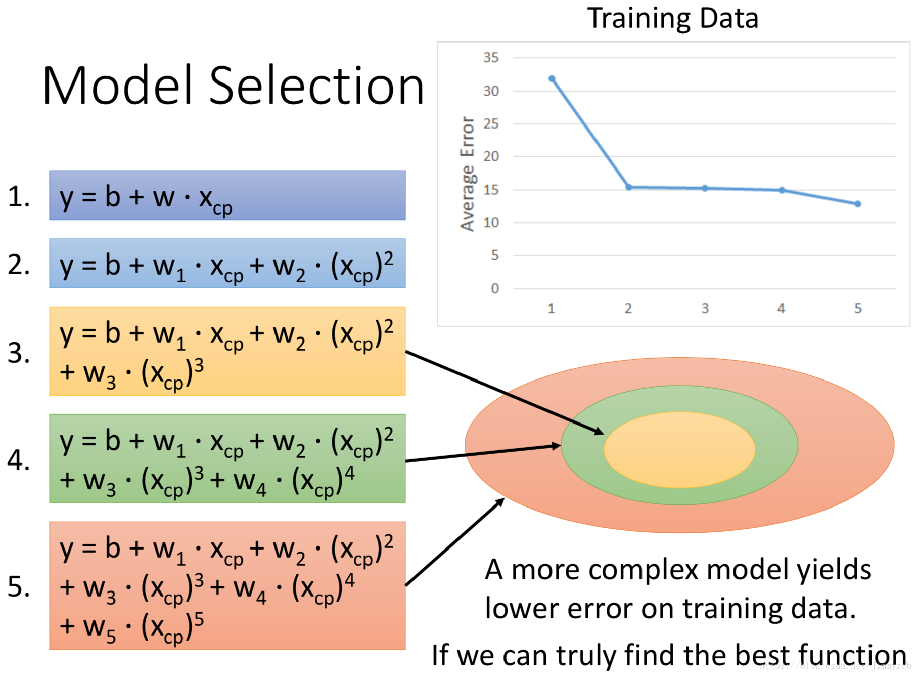

     

     当模型越复杂，训练集平均误差越低，如图可以直观地理解，在越复杂的模型（对应越大的集合）找到的best function拟合效果显然越好，但是测试集平均误差并不是单调递减，在引入4次、5次项之后反而急剧增大，此时产生了过拟合问题（可以尝试增加训练集样本来解决）。

     现在我们考虑更复杂的线性模型，即在Step1中的 f f <script type="math/tex" id="MathJax-Element-106">f</script>不再仅仅使用的xcp$x_{cp}$<script type="math/tex" id="MathJax-Element-107">x_{cp}</script>这一变量，引入变量 xs x s <script type="math/tex" id="MathJax-Element-108">x_s</script>（宝可梦种族），此时训练集平均误差为3.8，测试集平均误差为14.3，模型拟合与泛化效果都增强，在此基础上考虑变量的二次项，
     

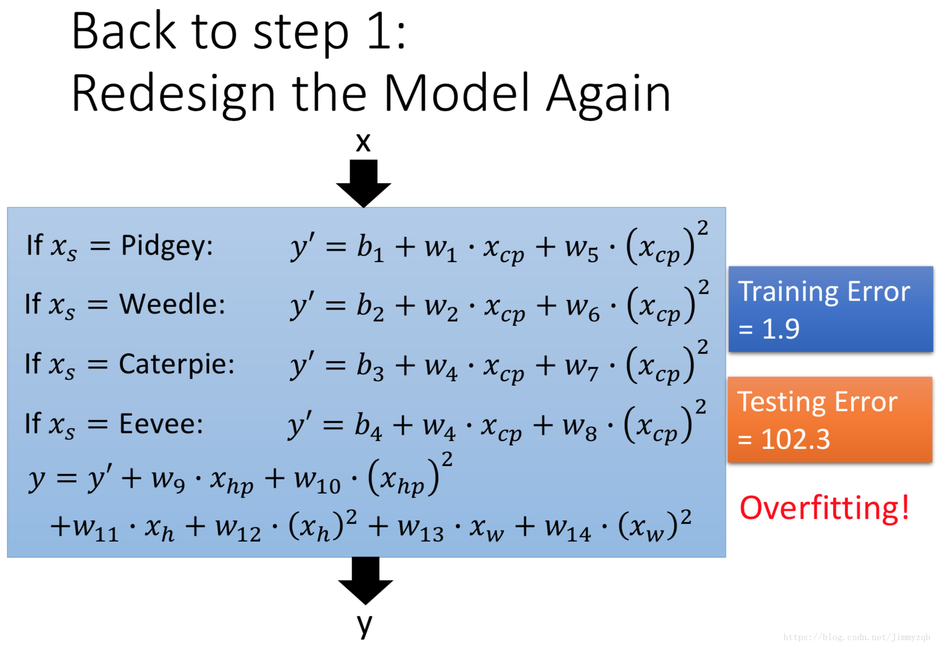
     此时模型过拟合，使用正则化方法来解决过拟合问题，即使Step2中的loss function 不仅仅考虑error，还考虑了参数个数， L=∑(ŷ n−(b+∑wxncp))2+λ∑(wi)2 L = ∑ ( y ^ n − ( b + ∑ w x c p n ) ) 2 + λ ∑ ( w i ) 2 <script type="math/tex" id="MathJax-Element-109">L = \sum(\hat{y}^n-(b+\sum wx_{cp}^n))^2+\lambda \sum (w_i)^2</script>，此时我们假设平滑的 f f <script type="math/tex" id="MathJax-Element-110">f</script>更接近真正的f∗$f^{\ast }$<script type="math/tex" id="MathJax-Element-111">f^*</script>。
     

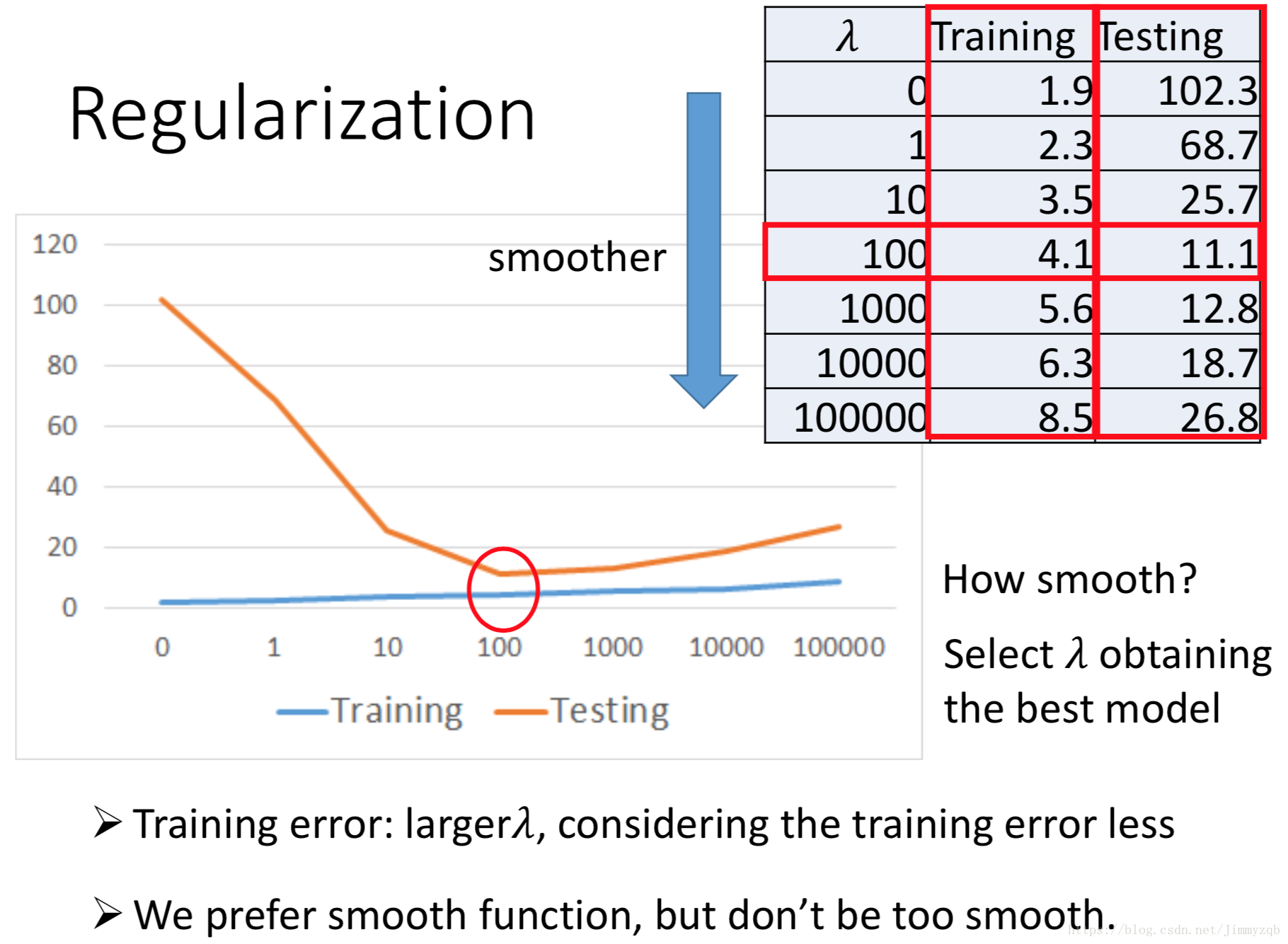
     为了兼顾最小化第二项，训练集平均误差相对于没有正则化的方法高，但是测试集平均误差降低，大大减少了过拟合的影响。

     <script type="math/tex" id="MathJax-Element-112">\quad</script>

     demo

     # 进化前后CP值数据
     x_data=[338.,333.,328.,207.,226.,25.,179.,60.,200.,606.]
     y_data=[640.,633.,619.,393.,428.,27.,193.,66.,226.,1591.]
     
     # 假设模型
     #y_data = b + w*x_data
     
     # 初始化w、b
     w,b = -4,-120
     # 学习速率
     lr = 0.000001
     # 迭代次数
     iter = 100000
     
     b_history=[b]
     w_history=[w]
     
     for i in range(iter):
         b_grad = 0.0
         w_grad = 0.0
         for n in range(len(x_data)):
             b_grad -= 2.0*(y_data[n] - b*w*x_data[n])*1.0
             w_grad -= 2.0*(y_data[n] - b*w*x_data[n])*x_data[n]
         # 更新参数
         b = b -lr*b_grad
         w = w -lr*w_grad
         # 储存w、b
         b_history.append(b)
         w_history.append(w)