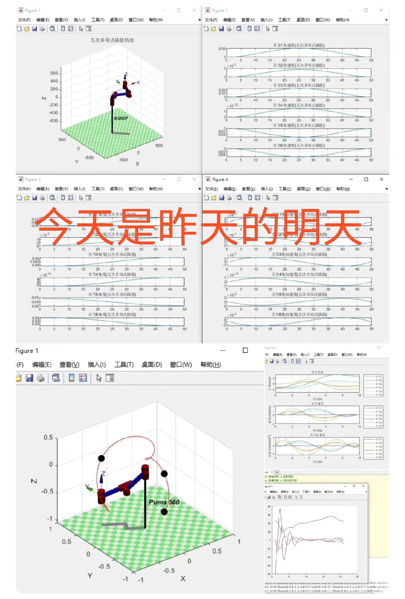
六自由度机械臂三套代码-三次/五次/七次多项式样条插值曲线、五次B样条曲线插值-2 轨迹规划，直线轨迹，圆弧轨迹，机器人工具箱，带源码注释。 起始点、中间点、终止点可自行修改。

在机器人领域，六自由度机械臂的轨迹规划是一项关键技术，它关乎机械臂能否高效、准确地完成各种任务。今天，咱就来唠唠基于三次/五次/七次多项式样条插值曲线以及五次B样条曲线插值的轨迹规划，还会涉及直线轨迹和圆弧轨迹，并借助机器人工具箱，同时附上源码注释，让大家能更好地理解。

三次多项式样条插值曲线

三次多项式样条插值常用于在给定起始点、中间点和终止点的情况下，生成平滑的轨迹。

import numpy as np
import matplotlib.pyplot as plt

# 定义起始点、中间点和终止点
start = np.array([0, 0])
mid = np.array([5, 5])
end = np.array([10, 0])

# 三次多项式系数计算函数
def cubic_spline_coeffs(p0, p1, t0, t1):
    h = t1 - t0
    A = np.array([
        [t0**3, t0**2, t0, 1],
        [t1**3, t1**2, t1, 1],
        [3*t0**2, 2*t0, 1, 0],
        [3*t1**2, 2*t1, 1, 0]
    ])
    B = np.array([p0[0], p1[0], 0, 0])
    coeffs_x = np.linalg.solve(A, B)

    B = np.array([p0[1], p1[1], 0, 0])
    coeffs_y = np.linalg.solve(A, B)
    return coeffs_x, coeffs_y

# 生成时间序列
t = np.linspace(0, 1, 100)

# 计算系数
coeffs_x1, coeffs_y1 = cubic_spline_coeffs(start, mid, 0, 0.5)
coeffs_x2, coeffs_y2 = cubic_spline_coeffs(mid, end, 0.5, 1)

# 计算轨迹点
x1 = coeffs_x1[0] * t[t < 0.5]**3 + coeffs_x1[1] * t[t < 0.5]**2 + coeffs_x1[2] * t[t < 0.5] + coeffs_x1[3]
y1 = coeffs_y1[0] * t[t < 0.5]**3 + coeffs_y1[1] * t[t < 0.5]**2 + coeffs_y1[2] * t[t < 0.5] + coeffs_y1[3]

x2 = coeffs_x2[0] * t[t >= 0.5]**3 + coeffs_x2[1] * t[t >= 0.5]**2 + coeffs_x2[2] * t[t >= 0.5] + coeffs_x2[3]
y2 = coeffs_y2[0] * t[t >= 0.5]**3 + coeffs_y2[1] * t[t >= 0.5]**2 + coeffs_y2[2] * t[t >= 0.5] + coeffs_y2[3]

x = np.concatenate((x1, x2))
y = np.concatenate((y1, y2))

# 绘制轨迹
plt.plot(x, y, label='Cubic Spline')
plt.scatter([start[0], mid[0], end[0]], [start[1], mid[1], end[1]], color='red', label='Control Points')
plt.legend()
plt.show()

代码分析：

• 首先定义了起始点 start、中间点 mid 和终止点 end。
• cubicsplinecoeffs 函数通过构建方程组并求解来得到三次多项式的系数。这里利用了矩阵运算，将时间和位置信息构建成矩阵 A 和向量 B，然后使用 np.linalg.solve 求解系数。
• 接着生成时间序列 t，并分两段计算系数和轨迹点，最后将两段轨迹连接起来并绘制。

五次多项式样条插值曲线

五次多项式样条相比三次多项式，能提供更平滑的轨迹，因为它有更多的系数可以调整。

# 五次多项式系数计算函数
def quintic_spline_coeffs(p0, p1, v0, v1, a0, a1, t0, t1):
    h = t1 - t0
    A = np.array([
        [t0**5, t0**4, t0**3, t0**2, t0, 1],
        [t1**5, t1**4, t1**3, t1**2, t1, 1],
        [5*t0**4, 4*t0**3, 3*t0**2, 2*t0, 1, 0],
        [5*t1**4, 4*t1**3, 3*t1**2, 2*t1, 1, 0],
        [20*t0**3, 12*t0**2, 6*t0, 2, 0, 0],
        [20*t1**3, 12*t1**2, 6*t1, 2, 0, 0]
    ])
    B = np.array([p0[0], p1[0], v0[0], v1[0], a0[0], a1[0]])
    coeffs_x = np.linalg.solve(A, B)

    B = np.array([p0[1], p1[1], v0[1], v1[1], a0[1], a1[1]])
    coeffs_y = np.linalg.solve(A, B)
    return coeffs_x, coeffs_y

# 假设初始和终点速度、加速度为0
v0 = np.array([0, 0])
v1 = np.array([0, 0])
a0 = np.array([0, 0])
a1 = np.array([0, 0])

# 计算系数
coeffs_x1, coeffs_y1 = quintic_spline_coeffs(start, mid, v0, v1, a0, a1, 0, 0.5)
coeffs_x2, coeffs_y2 = quintic_spline_coeffs(mid, end, v0, v1, a0, a1, 0.5, 1)

# 计算轨迹点
x1 = coeffs_x1[0] * t[t < 0.5]**5 + coeffs_x1[1] * t[t < 0.5]**4 + coeffs_x1[2] * t[t < 0.5]**3 + coeffs_x1[3] * t[t < 0.5]**2 + coeffs_x1[4] * t[t < 0.5] + coeffs_x1[5]
y1 = coeffs_y1[0] * t[t < 0.5]**5 + coeffs_y1[1] * t[t < 0.5]**4 + coeffs_y1[2] * t[t < 0.5]**3 + coeffs_y1[3] * t[t < 0.5]**2 + coeffs_y1[4] * t[t < 0.5] + coeffs_y1[5]

x2 = coeffs_x2[0] * t[t >= 0.5]**5 + coeffs_x2[1] * t[t >= 0.5]**4 + coeffs_x2[2] * t[t >= 0.5]**3 + coeffs_x2[3] * t[t >= 0.5]**2 + coeffs_x2[4] * t[t >= 0.5] + coeffs_x2[5]
y2 = coeffs_y2[0] * t[t >= 0.5]**5 + coeffs_y2[1] * t[t >= 0.5]**4 + coeffs_y2[2] * t[t >= 0.5]**3 + coeffs_y2[3] * t[t >= 0.5]**2 + coeffs_y2[4] * t[t >= 0.5] + coeffs_y2[5]

x = np.concatenate((x1, x2))
y = np.concatenate((y1, y2))

# 绘制轨迹
plt.plot(x, y, label='Quintic Spline')
plt.scatter([start[0], mid[0], end[0]], [start[1], mid[1], end[1]], color='red', label='Control Points')
plt.legend()
plt.show()

代码分析：

• quinticsplinecoeffs 函数构建了一个六阶的方程组来求解五次多项式的系数。相比三次多项式，多了初始和终点的速度、加速度信息作为约束条件。
• 同样假设初始和终点速度、加速度为0，分两段计算系数和轨迹点，最后绘制出五次多项式样条插值的轨迹。

七次多项式样条插值曲线

七次多项式样条有更多的自由度，能进一步优化轨迹的平滑性。

# 七次多项式系数计算函数
def septic_spline_coeffs(p0, p1, v0, v1, a0, a1, j0, j1, t0, t1):
    h = t1 - t0
    A = np.array([
        [t0**7, t0**6, t0**5, t0**4, t0**3, t0**2, t0, 1],
        [t1**7, t1**6, t1**5, t1**4, t1**3, t1**2, t1, 1],
        [7*t0**6, 6*t0**5, 5*t0**4, 4*t0**3, 3*t0**2, 2*t0, 1, 0],
        [7*t1**6, 6*t1**5, 5*t1**4, 4*t1**3, 3*t1**2, 2*t1, 1, 0],
        [42*t0**5, 30*t0**4, 20*t0**3, 12*t0**2, 6*t0, 2, 0, 0],
        [42*t1**5, 30*t1**4, 20*t1**3, 12*t1**2, 6*t1, 2, 0, 0],
        [210*t0**4, 120*t0**3, 60*t0**2, 24*t0, 6, 0, 0, 0],
        [210*t1**4, 120*t1**3, 60*t1**2, 24*t1, 6, 0, 0, 0]
    ])
    B = np.array([p0[0], p1[0], v0[0], v1[0], a0[0], a1[0], j0[0], j1[0]])
    coeffs_x = np.linalg.solve(A, B)

    B = np.array([p0[1], p1[1], v0[1], v1[1], a0[1], a1[1], j0[1], j1[1]])
    coeffs_y = np.linalg.solve(A, B)
    return coeffs_x, coeffs_y

# 假设初始和终点速度、加速度、加加速度为0
j0 = np.array([0, 0])
j1 = np.array([0, 0])

# 计算系数
coeffs_x1, coeffs_y1 = septic_spline_coeffs(start, mid, v0, v1, a0, a1, j0, j1, 0, 0.5)
coeffs_x2, coeffs_y2 = septic_spline_coeffs(mid, end, v0, v1, a0, a1, j0, j1, 0.5, 1)

# 计算轨迹点
x1 = coeffs_x1[0] * t[t < 0.5]**7 + coeffs_x1[1] * t[t < 0.5]**6 + coeffs_x1[2] * t[t < 0.5]**5 + coeffs_x1[3] * t[t < 0.5]**4 + coeffs_x1[4] * t[t < 0.5]**3 + coeffs_x1[5] * t[t < 0.5]**2 + coeffs_x1[6] * t[t < 0.5] + coeffs_x1[7]
y1 = coeffs_y1[0] * t[t < 0.5]**7 + coeffs_y1[1] * t[t < 0.5]**6 + coeffs_y1[2] * t[t < 0.5]**5 + coeffs_y1[3] * t[t < 0.5]**4 + coeffs_y1[4] * t[t < 0.5]**3 + coeffs_y1[5] * t[t < 0.5]**2 + coeffs_y1[6] * t[t < 0.5] + coeffs_y1[7]

x2 = coeffs_x2[0] * t[t >= 0.5]**7 + coeffs_x2[1] * t[t >= 0.5]**6 + coeffs_x2[2] * t[t >= 0.5]**5 + coeffs_x2[3] * t[t >= 0.5]**4 + coeffs_x2[4] * t[t >= 0.5]**3 + coeffs_x2[5] * t[t >= 0.5]**2 + coeffs_x2[6] * t[t >= 0.5] + coeffs_x2[7]
y2 = coeffs_y2[0] * t[t >= 0.5]**7 + coeffs_y2[1] * t[t >= 0.5]**6 + coeffs_y2[2] * t[t >= 0.5]**5 + coeffs_y2[3] * t[t >= 0.5]**4 + coeffs_y2[4] * t[t >= 0.5]**3 + coeffs_y2[5] * t[t >= 0.5]**2 + coeffs_y2[6] * t[t >= 0.5] + coeffs_y2[7]

x = np.concatenate((x1, x2))
y = np.concatenate((y1, y2))

# 绘制轨迹
plt.plot(x, y, label='Septic Spline')
plt.scatter([start[0], mid[0], end[0]], [start[1], mid[1], end[1]], color='red', label='Control Points')
plt.legend()
plt.show()

代码分析：

• septicsplinecoeffs 函数构建了一个八阶的方程组，除了位置、速度、加速度外，还加入了初始和终点的加加速度（jerk）信息来求解七次多项式的系数。
• 同样假设相关初始和终点条件为0，分两段计算并绘制轨迹，七次多项式通常能让轨迹在高阶导数上也更加平滑。

五次B样条曲线插值

B样条曲线以其局部控制性和良好的形状调配能力而受到青睐。

from scipy.interpolate import splev, splprep

# 控制点
points = np.array([start, mid, end])

# 计算B样条曲线
tck, u = splprep(points.T, w=None, k=5, s=0)

# 生成曲线上的点
u_new = np.linspace(u.min(), u.max(), 100)
x_new, y_new = splev(u_new, tck)

# 绘制轨迹
plt.plot(x_new, y_new, label='五次B样条曲线')
plt.scatter(points[:,0], points[:,1], color='red', label='Control Points')
plt.legend()
plt.show()

代码分析：

• 利用 scipy.interpolate 库中的 splprep 函数来计算五次B样条曲线的参数 tck 和节点向量 u。这里 k=5 表示五次B样条。
• 然后通过 splev 函数在新的参数值 u_new 上计算曲线上的点，最后绘制出五次B样条曲线和控制点。

直线轨迹规划

直线轨迹规划相对简单，直接在起始点和终止点之间进行线性插值。

# 直线轨迹
x_line = np.linspace(start[0], end[0], 100)
y_line = np.linspace(start[1], end[1], 100)

# 绘制轨迹
plt.plot(x_line, y_line, label='直线轨迹')
plt.scatter([start[0], end[0]], [start[1], end[1]], color='red', label='Control Points')
plt.legend()
plt.show()

代码分析：

• 使用 np.linspace 函数在起始点和终止点的坐标之间生成等