BEVFormer 介绍

BEVFormer 是今年中稿 ECCV 2022 的一篇论文。该篇论文提出了一个采用纯视觉（camera）做感知任务的算法模型 BEVFormer。BEVFormer 通过提取环视相机采集到的图像特征，并将提取的环视特征通过模型学习的方式转换到 BEV 空间（模型去学习如何将特征从 图像坐标系转换到 BEV 坐标系），从而实现 3D 目标检测和地图分割任务，并取得了 SOTA 的效果。

论文链接：https://arxiv.org/pdf/2203.17270.pdf

BEV感知介绍

这里我就不对bev感知进行过多的介绍和讲解了。想要系统了解学习BEV感知的，我推荐去看看深蓝学院的《BEV感知理论与实践》课程，这里面由历任百度自动驾驶高级算法专家傅东旭和前小鹏汽车自动驾驶AI团队负责人刘兰个川，两位行业资深专家亲自授课。全面梳理BEV感知算法及其发展脉络，细致讲解各类代表性算法的代码实现，并分享BEV落地的工程实践经验。

感兴趣的朋友可以直接点击下方链接，去了解一下：

BEV感知理论与实践 - 深蓝学院 - 专注人工智能与自动驾驶的学习平台www.shenlanxueyuan.com/channel/wYpdcYK9C9/detail

BEVFormer 的 Pipeline

根据自己调试算法模型以及对论文的理解，我这里将 BEVFormer 的 Pipeline 分成一下几个部分：

• Backbone + Neck （ResNet-101-DCN + FPN）提取环视图像的多尺度特征；
• 论文提出的 Encoder 模块（包括 Temporal Self-Attention 模块和 Spatial Cross-Attention 模块）完成环视图像特征向 BEV 特征的建模；
• 类似 Deformable DETR 的 Decoder 模块完成 3D 目标检测的分类和定位任务；
• 正负样本的定义（采用 Transformer 中常用的匈牙利匹配算法，Focal Loss + L1 Loss 的总损失和最小）；
• 损失的计算（Focal Loss 分类损失 + L1 Loss 回归损失）；
• 反向传播，更新网络模型参数；

接下来我将从输入数据格式，网络特征提取，BEV特征产生，BEV 特征解码完成 3D 框预测、正负样本定义、损失计算这六个方面完成 BEVFormer 的解析；

输入数据格式

对于 BEVFormer 网络模型而言，输入的数据是一个 6 维的张量：（bs，queue，cam，C，H，W）；

• bs：batch size 大小；
• queue：连续帧的个数；由于 BEVFormer 采用了时序信息的思想（我认为加入时序信息后，可以一定程度上缓解遮挡问题），所以输入到网络模型中的数据要包含除当前帧之外，之前几帧的数据；
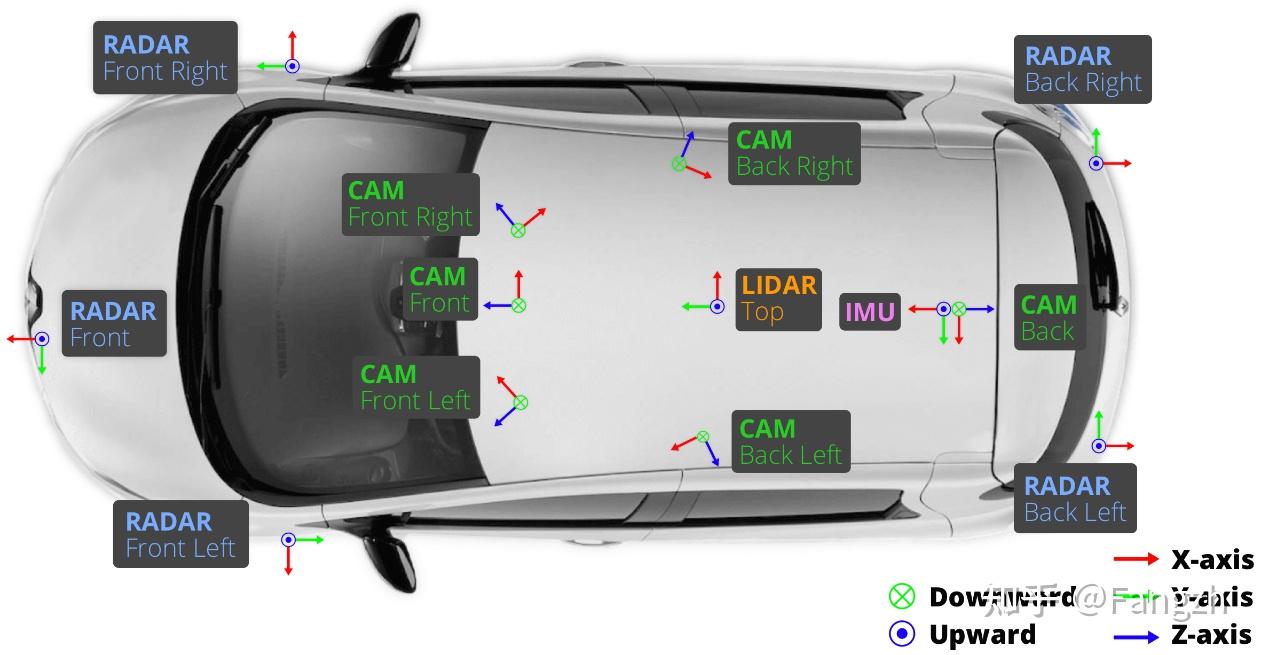
• cam：每帧中包含的图像数量，对于nuScenes数据集而言，由于一辆车带有六个环视相机传感器，可以实现 360° 全场景的覆盖，所以一帧会包含六个环视相机拍摄到的六张环视图片；
• C，H，W：图片的通道数，图片的高度，图片的宽度；

网络特征提取

网络特征提取的目的是将每一帧对应的六张环视图像的特征提取出来，便于后续转换到 BEV 特征空间，生成 BEV 特征，在特征提取过程中，张量流的变换情况如下：

# 输入图片信息 tensor: (bs, queue, cam, c, h, w)
# 通过 for loop 方式一次获取单帧对应的六张环视图像
# 送入到 Backbone + Neck 网络提取多尺度的图像特征

for idx in range(tensor.size(1) - 1): # 利用除当前帧之外的所有帧迭代计算 prev_bev 特征
single_frame = tensor[:, idx, :] # (bs, cam, c, h, w)

<span class="c1"># 将 bs * cam 看作是 batch size，将原张量 reshape 成 4 维的张量</span>
<span class="c1"># 待 Backbone + Neck 网络提取多尺度特征后，再把 bs * cam 的维度再拆成 bs，cam</span>

<span class="n">single_frame</span> <span class="o">=</span> <span class="n">single_frame</span><span class="o">.</span><span class="n">reshape</span><span class="p">(</span><span class="n">bs</span> <span class="o">*</span> <span class="n">cam</span><span class="p">,</span> <span class="n">c</span><span class="p">,</span> <span class="n">h</span><span class="p">,</span> <span class="n">w</span><span class="p">)</span>
<span class="n">feats</span> <span class="o">=</span> <span class="n">Backbone</span><span class="p">(</span><span class="n">FPN</span><span class="p">(</span><span class="n">single_frame</span><span class="p">))</span> 

<span class="s2">""" feats 是一个多尺度的特征列表 """</span>
<span class="p">[</span><span class="mi">0</span><span class="p">]:</span> <span class="p">(</span><span class="n">bs</span><span class="p">,</span> <span class="n">cam</span><span class="p">,</span> <span class="mi">256</span><span class="p">,</span> <span class="n">h</span> <span class="o">/</span> <span class="mi">8</span><span class="p">,</span> <span class="n">w</span> <span class="o">/</span> <span class="mi">8</span><span class="p">)</span>
<span class="p">[</span><span class="mi">1</span><span class="p">]:</span> <span class="p">(</span><span class="n">bs</span><span class="p">,</span> <span class="n">cam</span><span class="p">,</span> <span class="mi">256</span><span class="p">,</span> <span class="n">h</span> <span class="o">/</span> <span class="mi">16</span><span class="p">,</span> <span class="n">w</span> <span class="o">/</span> <span class="mi">16</span><span class="p">)</span>
<span class="p">[</span><span class="mi">2</span><span class="p">]:</span> <span class="p">(</span><span class="n">bs</span><span class="p">,</span> <span class="n">cam</span><span class="p">,</span> <span class="mi">256</span><span class="p">,</span> <span class="n">h</span> <span class="o">/</span> <span class="mi">32</span><span class="p">,</span> <span class="n">w</span> <span class="o">/</span> <span class="mi">32</span><span class="p">)</span>
<span class="p">[</span><span class="mi">3</span><span class="p">]:</span> <span class="p">(</span><span class="n">bs</span><span class="p">,</span> <span class="n">cam</span><span class="p">,</span> <span class="mi">256</span><span class="p">,</span> <span class="n">h</span> <span class="o">/</span> <span class="mi">64</span><span class="p">,</span> <span class="n">w</span> <span class="o">/</span> <span class="mi">64</span><span class="p">)</span></code></pre></div><h2 id="h_543335939_5" data-into-catalog-status="">BEV 特征产生</h2><p data-pid="ce6K5TVk">BEV 特征的产生用到的就是论文中最核心的部分 —— Encoder 模块，对应的网络结构如下：</p><figure data-size="normal"><div><img src="https://pic4.zhimg.com/v2-65a11a98d73c1111bcc05e1f10848195_1440w.jpg" data-size="normal" data-rawwidth="1015" data-rawheight="388" data-original-token="v2-ed46bd5a4188381f7e995f2d449d3c37" class="origin_image zh-lightbox-thumb" width="1015" data-original="https://pic4.zhimg.com/v2-65a11a98d73c1111bcc05e1f10848195_r.jpg"></div><figcaption>红色框代表 BEVFormer 中的 Encoder 模块</figcaption></figure><p data-pid="fAxTvFIl">Encoder 模块包含两个子模块 <u>Temporal Self-Attention模块</u> 以及 <u>Spatial Cross-Attention模块</u>；接下来我会分别介绍一下这两个模块；</p><p data-pid="01593OLl">在梳理具体的代码实现之前，首先介绍下在 <u>Temporal Self-Attention</u> 模块和 <u>Spatial Cross-Attention</u> 模块中都要用到的一个组件 —— 多尺度的可变形注意力模块；这个模块是将 Transformer 的全局注意力变为局部注意力的一个非常关键的组件，用于减少训练时间，提高 Transformer 的收敛速度；（该思想最早出现在 Deformable DETR 中）</p><p data-pid="ZqKkGSXl">在代码中，多尺度可变形注意力模块是以 CUDA 扩展的形式进行封装的，实现逻辑也是在 CUDA 代码中；这里放一下代码链接；</p><ul><li data-pid="F_THYTdC"><a href="https://link.zhihu.com/?target=https%3A//github.com/open-mmlab/mmcv/blob/master/mmcv/ops/csrc/pytorch/cuda/ms_deform_attn_cuda.cu" class=" external" target="_blank" rel="nofollow noreferrer"><span class="invisible">https://</span><span class="visible">github.com/open-mmlab/m</span><span class="invisible">mcv/blob/master/mmcv/ops/csrc/pytorch/cuda/ms_deform_attn_cuda.cu</span><span class="ellipsis"></span></a></li><li data-pid="Se7Kh_36"><a href="https://link.zhihu.com/?target=https%3A//github.com/open-mmlab/mmcv/blob/master/mmcv/ops/csrc/common/cuda/ms_deform_attn_cuda_kernel.cuh" class=" external" target="_blank" rel="nofollow noreferrer"><span class="invisible">https://</span><span class="visible">github.com/open-mmlab/m</span><span class="invisible">mcv/blob/master/mmcv/ops/csrc/common/cuda/ms_deform_attn_cuda_kernel.cuh</span><span class="ellipsis"></span></a></li></ul><p data-pid="CSt-MWlQ">基于我所调试的代码以及自己的思考，简单概括下<u>多尺度的可变形注意力</u>模块对数据处理的Pipeline，概括如下：</p><figure data-size="normal"><div><img src="https://pica.zhimg.com/v2-5ef798d620bbb9d1ec9b9d9f22c3739c_1440w.jpg" data-size="normal" data-rawwidth="1194" data-rawheight="495" data-original-token="v2-843220515717ee478b0f3eb0b9b47313" class="origin_image zh-lightbox-thumb" width="1194" data-original="https://pica.zhimg.com/v2-5ef798d620bbb9d1ec9b9d9f22c3739c_r.jpg"></div><figcaption>Deformable Attention 模块 Pipeline</figcaption></figure><p data-pid="3jw1uaKV">通过流程图可知，输入到 Deformable Attention Module CUDA 扩展的变量主要有五个，分别是<u>采样位置</u>（Sample Location）、<u>注意力权重</u>（Attention Weights）、<u>映射后的 Value 特征</u>、<u>多尺度特征每层特征起始索引位置</u>、<u>多尺度特征图的空间大小（便于将采样位置由归一化的值变成绝对位置）</u>；</p><p data-pid="sycH1NRi"><u>多尺度可变形注意力</u>模块与 Transformer 中常见的先生成 Attention Map，再计算加权和的方式不同；常规而言 Attention Map = Query 和 Key 做内积运算，将 Attention Map 再和 Value 做加权；但是由于这种方式计算量开销会比较大，所以在 Deformable DETR 中用局部注意力机制代替了全局注意力机制，只对几个采样点进行采样，<b>而采样点的位置相对于参考点的偏移量和每个采样点在加权时的比重均是靠 Query 经过 Linear 层学习得到的</b>。</p><p data-pid="d3uE3ZmQ">各个变量在 <u>Temporal Self-Attention</u> 模块、<u>Spatial Cross-Attention</u> 模块的作用会在后续进行系统分析，这里就是先笼统的说下我对这个 CUDA 扩展的理解，形成一种感性的认识。</p><h3 id="h_543335939_6" data-into-catalog-status=""><b>Temporal Self-Attention 模块</b></h3><ul><li data-pid="r_kMC_dq">功能</li></ul><p data-pid="w2d6F3E_">通过引入时序信息（插图中的 History BEV）与当前时刻的 BEV Query 进行融合，提高 BEV Query 的建模能力；</p><ul><li data-pid="1NVJSewb">代码实现</li></ul><p data-pid="75qsambp">对于 Temporal Self-Attention 模块而言，需要 bev_query、bev_pos、prev_bev、ref_point、value等参数（需要用到的参数参考 Deformable Attention Pipeline 图解）</p><p data-pid="-zfgOsQV">参数 <code>bev_query</code> </p><p data-pid="Uel7gun0">一个完全 <b>learnable parameter</b>，通过 nn.Embedding() 函数得到，形状 shape = (200 * 200，256)；200，200 分别代表 BEV 特征平面的长和宽；</p><p data-pid="SVSszSp3">参数 <code>bev_pose</code> </p><p data-pid="koPs7VAj">感觉也是一个完全 <b>learnable parameter</b>，与 2D 检测中常见的正余弦编码方式不同，感觉依旧是把不同的 grid 位置映射到一个高维的向量空间，shape = (bs，256，200，200）代码如下：</p><div class="highlight"><pre><code class="language-python3"><span class="s2">""" bev_pose 的生成过程 """</span>

# w, h 分别代表 bev 特征的空间尺寸 200 * 200
x = torch.arange(w, device=mask.device)
y = torch.arange(h, device=mask.device)

# self.col_embed 和 self.row_embed 分别是两个 Linear 层，将(200, )的坐标向高维空间做映射
x_embed = self.col_embed(x) # (200, 128)
y_embed = self.row_embed(y) # (200, 128)

# pos shape: (bs, 256, 200, 200)
pos = torch.cat((x_embed.unsqueeze(0).repeat(h, 1, 1), y_embed.unsqueeze(1).repeat(1, w, 1)), dim=-1).permute(2, 0, 1).unsqueeze(0).repeat(mask.shape[0], 1, 1, 1)

参数 ref_point

这个参数根据当前 Temporal Self-Attention 模块是否有 prev_bev 特征输入而言，会对应不同的情况，之所以会出现不同，是考虑到了前后时刻 BEV 特征存在特征不对齐的问题，BEV 特征不对齐主要体现在以下两个方面。

一、车自身是不断运动的

上一时刻和当前时刻，由于车自身的不断运动，两个时刻的 BEV 特征在空间上是不对齐的；针对这一问题，为了实现两个时刻特征的空间对齐，需要用到 can_bus 数据中有关车自身旋转角度和偏移的信息，从而对上一时刻的 BEV 特征与当前时刻的 BEV 特征在空间上实现特征对齐；

二、车周围的物体也在一定范围内运动

针对车周围的物体可能在不同时刻也有移动，这部分的特征对齐就是靠网络自身的注意力模块去学习实现修正了。

综上，对于 Temporal Self-Attention 模块没有输入 prev_bev（第一帧没有前一时刻的 BEV 特征）的情况，其 ref_point = ref_2d；对于存在输入 prev_bev 的情况，其 ref_point = ref_2d + shift；

涉及到的ref_2d、shift参数，核心代码如下：

“”“shift 参数的生成”“”

obtain rotation angle and shift with ego motion

delta_x = kwargs[‘img_metas’][0][‘can_bus’][0]
delta_y = kwargs[‘img_metas’][0][‘can_bus’][1]
ego_angle = kwargs[‘img_metas’][0][‘can_bus’][-2] / np.pi * 180
rotation_angle = kwargs[‘img_metas’][0][‘can_bus’][-1]
grid_length_y = grid_length[0]
grid_length_x = grid_length[1]
translation_length = np.sqrt(delta_x ** 2 + delta_y ** 2)
translation_angle = np.arctan2(delta_y, delta_x) / np.pi * 180
if translation_angle < 0:
translation_angle += 360
bev_angle = ego_angle - translation_angle
shift_y = translation_length *
np.cos(bev_angle / 180 * np.pi) / grid_length_y / bev_h
shift_x = translation_length *
np.sin(bev_angle / 180 * np.pi) / grid_length_x / bev_w
shift_y = shift_y * self.use_shift
shift_x = shift_x * self.use_shift
shift = bev_queries.new_tensor([shift_x, shift_y]) # shape (2,)

通过旋转和平移变换实现 BEV 特征的对齐，对于平移部分是通过对参考点加上偏移量shift体现的

if prev_bev is not None:
if prev_bev.shape[1] == bev_h * bev_w:
prev_bev = prev_bev.permute(1, 0, 2)
if self.rotate_prev_bev:
num_prev_bev = prev_bev.size(1)
prev_bev = prev_bev.reshape(bev_h, bev_w, -1).permute(2, 0, 1) # sequence -> grid
prev_bev = rotate(prev_bev, rotation_angle, center=self.rotate_center)
prev_bev = prev_bev.permute(1, 2, 0).reshape(bev_h * bev_w, num_prev_bev, -1)

“”“ref_2d 参数的生成，常规的 2D 网格生成的规则坐标点”“”
ref_y, ref_x = torch.meshgrid(torch.linspace(0.5, H - 0.5, H, dtype=dtype, device=device),
torch.linspace(0.5, W - 0.5, W, dtype=dtype, device=device))
ref_y = ref_y.reshape(-1)[None] / H
ref_x = ref_x.reshape(-1)[None] / W
ref_2d = torch.stack((ref_x, ref_y), -1)
ref_2d = ref_2d.repeat(bs, 1, 1).unsqueeze(2)

参数 value

参数 value 就是对应着bev_query去查询的特征；

对于 Temporal Self-Attention 模块输入包含 prev_bev时，value = [prev_bev，bev_query]，对应的参考点 ref_point = [ref_2d + shift，ref_2d]；如果输入不包含 prev_bev时，value = [bev_query，bev_query]，对应的参考点ref_point = [ref_2d，ref_2d]。

相应的，之前介绍的 bev_query 在输入包含 prev_bev时，bev_query = [value[0]，bev_query]；输入不包含 prev_bev时，value = [bev_query，bev_query]；

整体的思路还是计算在计算 self-attention，无论是否存在prev_bev，都是在计算prev_bev以及bev_query自身的相似性，最后将两组计算得到的bev_query结果做一下平均。

内部参数 Offset、Weights、 Sample Location

参数Offset的计算是同时考虑了value[0]和bev_query的信息，在映射空间的维度上进行了concat，并基于 concat 后的特征，去计算 Offset以及attention weights ，涉及到的核心代码如下，这里解释一下为什么 level = 1，由于 BEV 特征只有一层，所以只会对一层 200 * 200 空间大小的 BEV 特征，基于每个位置采样四个点，重新构造新的 BEV 特征；

“”" bev_query 按照通道维度进行 concat “”"

query = torch.cat([value[0:1], query], -1)  # (bs, 40000, 512)

“”" value 经过 Linear 做映射 “”"
value = self.value_proj(value)

“”" offsets 以及 attention weights 的生成过程 “”"
# sampling_offsets: shape = (bs, num_query, 8, 1, 4, 2)
# 对 query 进行维度映射得到采样点的偏移量
sampling_offsets = self.sampling_offsets(query).view(bs, num_query, self.num_heads, self.num_levels, self.num_points, 2)

# 对 query 进行维度映射得到注意力权重
attention_weights = self.attention_weights(query).view(bs, num_query, self.num_heads, self.num_levels * self.num_points)
attention_weights = attention_weights.softmax(-1)

# attention_weights: shape = (bs, num_query, 8, 1, 4)
attention_weights = attention_weights.view(bs, num_query, self.num_heads, self.num_levels, self.num_points)

“”" sample location 的生成过程
通过代码可以观察到两点：
1. 通过 query 学到的 sampling_offsets 偏移量是一个绝对量，不是相对量，所以需要做 normalize；
2. 最终生成的 sampling_locations 是一个相对量；
“”“
offset_normalizer = torch.stack([spatial_shapes[…, 1], spatial_shapes[…, 0]], -1)
sampling_locations = reference_points[:, :, None, :, None, :]
+ sampling_offsets / offset_normalizer[None, None, None, :, None, :]

输出bev query

”“” 各个参数的 shape 情况

1. value: (2，40000，8，32） # 2: 代表前一时刻的 BEV 特征和后一时刻的 BEV 特征，两个特征在计算的过程中是互不干扰的，

                             # 40000: 代表 bev_query 200 * 200 空间大小的每个位置

                             # 8: 代表8个头，# 32: 每个头表示为 32 维的特征

2. spatial_shapes: (200, 200) # 方便将归一化的 sampling_locations 反归一化

3. level_start_index: 0 # BEV 特征只有一层

4. sampling_locations: (2, 40000, 8, 1, 4, 2)

5. attention_weights: (2, 40000, 8, 1, 4)



6. output: (2, 40000, 8, 32)

“”"

output = MultiScaleDeformableAttnFunction.apply(value,

spatial_shapes,

level_start_index,

sampling_locations,

attention_weights,

self.im2col_step)

“”" 最后将前一时刻的 bev_query 与当前时刻的 bev_query 做平均
output = output.permute(1, 2, 0)
output = (output[…, :bs] + output[…, bs:])/self.num_bev_queue

至此，Temporal Self-Attention 模块的逻辑到此结束，将生成的 bev_query 送入到后面的 Spatial Cross-Attention 模块中。

Spatial Cross-Attention 模块

• 功能

利用 Temporal Self-Attention 模块输出的 bev_query， 对主干网络和 Neck 网络提取到的多尺度环视图像特征进行查询，生成 BEV 空间下的BEV Embedding特征；

• 代码实现

对于 Spatial Cross-Attention 模块而言，与 Temporal Self-Attention 模块需要的参数很类似，但是并不需要 bev_pos 参数，只需要 bev_query、ref_point、value（就是 concat 到一起的多尺度特征）；虽不需要 bev_pose，但是整体流程与 Deformable Attention Pipeline 图解类似

参数bev_query

bev_query参数来自于 Temporal Self-Attention 模块的输出；

参数value

对于 Transformer 而言，由于其本身是处理文本序列的模型，而文本序列都是一组组一维的数据，所以需要将前面提取的多尺度特征做 flatten() 处理，并将所有层的特征汇聚到一起，方便之后做查询；对应的核心代码如下：

“”" 首先将多尺度的特征每一层都进行 flatten() “”"

for lvl, feat in enumerate(mlvl_feats):

bs, num_cam, c, h, w = feat.shape

spatial_shape = (h, w)

feat = feat.flatten(3).permute(1, 0, 3, 2)

if self.use_cams_embeds:

feat = feat + self.cams_embeds[:, None, None, :].to(feat.dtype)

feat = feat + self.level_embeds[None, None, lvl:lvl + 1, :].to(feat.dtype)

spatial_shapes.append(spatial_shape)

feat_flatten.append(feat)

“”" 对每个 camera 的所有层级特征进行汇聚 “”"
feat_flatten = torch.cat(feat_flatten, 2) # (cam, bs, sum(h*w), 256)
spatial_shapes = torch.as_tensor(spatial_shapes, dtype=torch.long, device=bev_pos.device)

# 计算每层特征的起始索引位置
level_start_index = torch.cat((spatial_shapes.new_zeros((1,)), spatial_shapes.prod(1).cumsum(0)[:-1]))

# 维度变换
feat_flatten = feat_flatten.permute(0, 2, 1, 3) # (num_cam, sum(H*W), bs, embed_dims)

参数ref_point

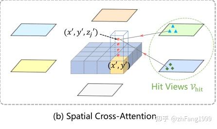
首先说一下ref_3d坐标点，这个ref_3d是基于 BEV 空间产生的三维空间规则网格点，同时在 z 轴方向上人为的选择了 4 个坐标点。

这里要使用 z 轴，并在 z 轴方向上采样的物理意义，我的理解是为了提取每个 BEV 位置处不同高度的特征；可以理解一下，假如对于 BEV 平面上的（x，y）处有一辆汽车，它所对应的特征应该由车底、车身、车顶处等位置的特征汇聚而成，但是这些位置对应的高度是不一致的，而为了更好的获取在 BEV 空间下的（x，y）处的特征，就将（x，y）的坐标进行了 lift ，从而将 BEV 坐标系下的三维点映射回图像平面后可以去查询并融合更加准确的特征；

而在映射的过程中，论文中也提到，由于每个参考点映射回图像坐标系后，不会落到六个图像上，只可能落在其中的某些图像的某些位置上，所以只对这些参考点附近的位置进行采样，可以提高模型的收敛速度（借鉴了 Deformable DETR 的思想）

ref_3d参数生成、3D 坐标向图像平面转换等过程的核心代码如下，真正用在 Spatial Cross-Attention 模块中的参考点是下面代码段中的reference_points_cam 。

“”" ref_3d 坐标生成 “”"

zs = torch.linspace(0.5, Z - 0.5, num_points_in_pillar, dtype=dtype, device=device).view(-1, 1, 1).expand(num_points_in_pillar, H, W) / Z

xs = torch.linspace(0.5, W - 0.5, W, dtype=dtype, device=device).view(1, 1, W).expand(num_points_in_pillar, H, W) / W

ys = torch.linspace(0.5, H - 0.5, H, dtype=dtype, device=device).view(1, H, 1).expand(num_points_in_pillar, H, W) / H

ref_3d = torch.stack((xs, ys, zs), -1)  # (4, 200, 200, 3)  (level, bev_h, bev_w, 3) 3代表 x,y,z 坐标值

ref_3d = ref_3d.permute(0, 3, 1, 2).flatten(2).permute(0, 2, 1)  # (4, 200 * 200, 3)

ref_3d = ref_3d[None].repeat(bs, 1, 1, 1)  # (1, 4, 200 * 200, 3)

“”" BEV 空间下的三维坐标点向图像空间转换的过程
代码中的lidar2img需要有两点需要注意

1. BEV 坐标系 这里指 lidar 坐标系
2. 这里提到的lidar2img是经过坐标变换的，一般分成三步
   第一步：lidar 坐标系 -> ego vehicle 坐标系
   第二步：ego vehicle 坐标系 -> camera 坐标系
   第三部：camera 坐标系 通过相机内参 得到像素坐标系
   以上这三步用到的所有平移和旋转矩阵都合并到了一起，形成了 lidar2img 旋转平移矩阵

同时需要注意：再与lidar2img矩阵乘完，还需要经过下面两步坐标系转换，才是得到了三维坐标点在二维图像平面上的点
“”"

(level, bs, cam, num_query, 4)

坐标系转换第一步：reference_points_cam = torch.matmul(lidar2img.to(torch.float32), reference_points.to(torch.float32)).squeeze(-1)
eps = 1e-5
bev_mask = (reference_points_cam[…, 2:3] > eps) # (level, bs, cam, num_query, 1)
坐标系转换第二步：reference_points_cam = reference_points_cam[…, 0:2] / torch.maximum(reference_points_cam[…, 2:3], torch.ones_like(reference_points_cam[…, 2:3]) * eps)

reference_points_cam = (bs, cam = 6, 40000, level = 4, xy = 2)

reference_points_cam[…, 0] /= img_metas[0][‘img_shape’][0][1] # 坐标归一化
reference_points_cam[…, 1] /= img_metas[0][‘img_shape’][0][0] # 坐标归一化

bev_mask 用于评判某一 三维坐标点 是否落在了 二维坐标平面上

bev_mask = (bs, cam = 6, 40000, level = 4)

bev_mask = (bev_mask & (reference_points_cam[…, 1:2] > 0.0)
& (reference_points_cam[…, 1:2] < 1.0)
& (reference_points_cam[…, 0:1] < 1.0)
& (reference_points_cam[…, 0:1] > 0.0))

需要注意的是，上述得到的bev_query以及reference_points_cam参数并不是直接用在了 Spatial Cross-Attention 模块中，而是选择了有用的部分进行使用（减少模型的计算量，提高训练过程的收敛速度），这里还是根据 Deformable Attention Pipeline 中涉及的参数进行说明：

参数queries_rebatch

之前也有提到，并不是 BEV 坐标系下的每个三维坐标都会映射到环视相机的所有图像上，而只会映射到其中的某几张图片上，所以使用所有来自 Temporal Self-Attention 模块的所有bev_query会消耗很大的计算量，所以这里是对bev_query进行了重新的整合，涉及的核心代码如下：

indexes = []

# 根据每张图片对应的bev_mask结果，获取有效query的index

for i, mask_per_img in enumerate(bev_mask):

index_query_per_img = mask_per_img[0].sum(-1).nonzero().squeeze(-1)

indexes.append(index_query_per_img)

queries_rebatch = query.new_zeros([bs self.num_cams, max_len, self.embed_dims])
reference_points_rebatch = reference_points_cam.new_zeros([bs self.num_cams, max_len, D, 2])

for i, reference_points_per_img in enumerate(reference_points_cam):
for j in range(bs):
index_query_per_img = indexes[i]

    <span class="c1"># 重新整合 `bev_query` 特征，记作 `query_rebatch</span>
    <span class="n">queries_rebatch</span><span class="p">[</span><span class="n">j</span> <span class="o">*</span> <span class="bp">self</span><span class="o">.</span><span class="n">num_cams</span> <span class="o">+</span> <span class="n">i</span><span class="p">,</span> <span class="p">:</span><span class="nb">len</span><span class="p">(</span><span class="n">index_query_per_img</span><span class="p">)]</span> <span class="o">=</span> <span class="n">query</span><span class="p">[</span><span class="n">j</span><span class="p">,</span> <span class="n">index_query_per_img</span><span class="p">]</span>

    <span class="c1"># 重新整合 `reference_point`采样位置，记作`reference_points_rebatch`</span>
    <span class="n">reference_points_rebatch</span><span class="p">[</span><span class="n">j</span> <span class="o">*</span> <span class="bp">self</span><span class="o">.</span><span class="n">num_cams</span> <span class="o">+</span> <span class="n">i</span><span class="p">,</span> <span class="p">:</span><span class="nb">len</span><span class="p">(</span><span class="n">index_query_per_img</span><span class="p">)]</span> <span class="o">=</span> <span class="n">reference_points_per_img</span><span class="p">[</span><span class="n">j</span><span class="p">,</span> <span class="n">index_query_per_img</span><span class="p">]</span></code></pre></div><p data-pid="eZtM3ujW">参数<code>reference_points_rebatch</code></p><p data-pid="NAuLgLgf">与产生<code>query_rebatch</code>的原因相同，获得映射到二维图像后的有效位置，对原有的<code>reference_points</code>进行重新的整合<code>reference_points_rebatch</code>。</p><p data-pid="hEaoCFab">内部参数<code>Offset</code>、<code>Weights</code>、<code>Sample Locations</code></p><div class="highlight"><pre><code class="language-python3"><span class="s2">""" 获取 sampling_offsets，依旧是对 query 做 Linear 做维度的映射，但是需要注意的是

这里的 query 指代的是上面提到的 quries_rebatch “”"
# sample 8 points for single ref point in each level.

# sampling_offsets: shape = (bs, max_len, 8, 4, 8, 2)
sampling_offsets = self.sampling_offsets(query).view(bs, num_query, self.num_heads, self.num_levels, self.num_points, 2)
attention_weights = self.attention_weights(query).view(bs, num_query, self.num_heads, self.num_levels * self.num_points)

attention_weights = attention_weights.softmax(-1)

# attention_weights: shape = (bs, max_len, 8, 4, 8)
attention_weights = attention_weights.view(bs, num_query,
self.num_heads,
self.num_levels,
self.num_points)

“”" 生成 sampling location “”"
offset_normalizer = torch.stack([spatial_shapes[…, 1], spatial_shapes[…, 0]], -1)

reference_points = reference_points[:, :, None, None, None, :, :]
sampling_offsets = sampling_offsets / offset_normalizer[None, None, None, :, None, :]
sampling_locations = reference_points + sampling_offsets

输出bev_embedding

将上述处理好的参数，送入到多尺度可变形注意力模块中生成bev_embedding特征；

“”"

1. value: shape = (cam = 6, sum(h_i * w_i) = 30825, head = 8, dim = 32)

2. spatial_shapes = ([[116, 200], [58, 100], [29,  50], [15,  25]])

3. level_start_index= [0, 23200, 29000, 30450]

4. sampling_locations = (cam, max_len, 8, 4, 8, 2)

5. attention_weights = (cam, max_len, 8, 4, 8)



6. output = (cam, max_len, 8, 32)

“”"

output = MultiScaleDeformableAttnFunction.apply(value, spatial_shapes, level_start_index, sampling_locations,

attention_weights, self.im2col_step)

“”“最后再将六个环视相机查询到的特征整合到一起，再求一个平均值 “””
for i, index_query_per_img in enumerate(indexes):
for j in range(bs): # slots: (bs, 40000, 256)
slots[j, index_query_per_img] += queries[j * self.num_cams + i, :len(index_query_per_img)]

count = bev_mask.sum(-1) > 0
count = count.permute(1, 2, 0).sum(-1)
count = torch.clamp(count, min=1.0)
slots = slots / count[…, None] # maybe normalize.
slots = self.output_proj(slots)

以上就是 Spatial Cross-Attention 模块的整体逻辑。

将 Temporal Self-Attetion 模块和 Spatial Cross-Attention 模块堆叠在一起，并重复六次，最终得到的 BEV Embedding 特征作为下游 3D 目标检测和道路分割任务的 BEV 空间特征。

Decoder模块

上述产生 BEV 特征的过程是用了当前输入到网络模型中除当前帧外，之前所有帧的特征去迭代修正去获得prev_bev的特征；所以在利用 Decoder 模块进行解码之前，需要对当前时刻环视的 6 张图片同样利用 Backbone + Neck 提取多尺度的特征，然后利用上述的 Temporal Self-Attention 模块和 Spatial Cross-Attention 模块的逻辑生成当前时刻的bev_embedding，然后将这部分特征送入到 Decoder 中进行 3D 目标检测。

下面分析 Decoder 模块是如何获得预测框和分类得分的。

• query、query_pos

首先是object_query_embed参数，该参数同样是沿用了 2D 目标检测中的 Deformable DETR 的思想。query和query_pose 全都是可学习的。模型直接用 nn.Embedding() 生成一组（900，512）维的张量。然后将 512 维的张量分成两组，分别构成了query = (900，256)和query_pos = (900，256) 。

• referece_points

之前介绍过，对于多尺度可变形注意力模块是需要参考点的，但是在预测过程中是没有参考点的，这就需要网络学习出来，网络是靠 query_pos学习得到的，核心代码如下：

reference_points = self.reference_points(query_pos)  # (bs, 900, 3)  3 代表 (x, y, z) 坐标

reference_points = reference_points.sigmoid()  # absolute -> relative

init_reference_out = reference_points 

• Decoder 逻辑

在获取到需要用到的query、query_pos、reference_points参数后，后面的逻辑有些类似 Deformabe DETR 的 Decoder 过程，简单概括如下几点：

1. 利用query和query_pos去做常规的 Self-Attention 运算更新query；
2. 利用 Self-Attention 得到的 query，之前获得的 bev_embedding作为value，query_pos，由 query生成的reference_points（虽然生成的x，y，z参考点位置，但是 BEV Embedding 是二维的，所以参考点只选择了前两维）仿照 Deformable Attention Module 的 pipeline 做可变形注意力；

可变形注意力核心代码如下：

“”" 由 query 生成 sampling_offsets 和 attention_weights “”"

sampling_offsets = self.sampling_offsets(query).view(

bs, num_query, self.num_heads, self.num_levels, self.num_points, 2)  # (bs, 900, 8, 1, 4, 2)

attention_weights = self.attention_weights(query).view(

bs, num_query, self.num_heads, self.num_levels * self.num_points)  # (bs, 900, 8, 4)

attention_weights = attention_weights.softmax(-1)

attention_weights = attention_weights.view(bs, num_query,

self.num_heads,

self.num_levels,

self.num_points)  # (bs, 900, 8, 1, 4)

“”" sampling_offsets 和 reference_points 得到 sampling_locations “”"
offset_normalizer = torch.stack(
[spatial_shapes[…, 1], spatial_shapes[…, 0]], -1)
sampling_locations = reference_points[:, :, None, :, None, :]
+ sampling_offsets
/ offset_normalizer[None, None, None, :, None, :]

“”" 多尺度可变形注意力模块 “”"

value: shape = (bs, 40000, 8, 32)

spatial_shapes = (200, 200)

level_start_index = 0

sampling_locations = (bs, 900, 8, 1, 4, 2)

attention_weights = (bs, 900, 8, 1, 4)

output = (bs, 900, 256)

output = MultiScaleDeformableAttnFunction.apply(value, spatial_shapes, level_start_index, sampling_locations,
attention_weights, self.im2col_step)

在获得查询到的特征后，会利用回归分支（FFN 网络）对提取的特征计算回归结果，预测 10 个输出；

我的理解这 10 个维度的含义为：[xc，yc，w，l，zc，h，rot.sin()，rot.cos()，vx，vy]；[预测框中心位置的x方向偏移，预测框中心位置的y方向偏移，预测框的宽，预测框的长，预测框中心位置的z方向偏移，预测框的高，旋转角的正弦值，旋转角的余弦值，x方向速度，y方向速度]；

然后根据预测的偏移量，对参考点的位置进行更新，为级联的下一个 Decoder 提高精修过的参考点位置，核心代码如下：

if reg_branches is not None:  # update the reference point.

tmp = reg_branches[lid](output)  # (bs, 900, 256) -> (bs, 900, 10) 回归分支的预测输出

assert reference_points.shape[-1] == 3

new_reference_points = torch.zeros_like(reference_points)
<span class="c1"># 预测出来的偏移量是绝对量</span>
<span class="n">new_reference_points</span><span class="p">[</span><span class="o">...</span><span class="p">,</span> <span class="p">:</span><span class="mi">2</span><span class="p">]</span> <span class="o">=</span> <span class="n">tmp</span><span class="p">[</span><span class="o">...</span><span class="p">,</span> <span class="p">:</span><span class="mi">2</span><span class="p">]</span> <span class="o">+</span> <span class="n">inverse_sigmoid</span><span class="p">(</span><span class="n">reference_points</span><span class="p">[</span><span class="o">...</span><span class="p">,</span> <span class="p">:</span><span class="mi">2</span><span class="p">])</span>  <span class="c1"># 框中心处的 x, y 坐标</span>
<span class="n">new_reference_points</span><span class="p">[</span><span class="o">...</span><span class="p">,</span> <span class="mi">2</span><span class="p">:</span><span class="mi">3</span><span class="p">]</span> <span class="o">=</span> <span class="n">tmp</span><span class="p">[</span><span class="o">...</span><span class="p">,</span> <span class="mi">4</span><span class="p">:</span><span class="mi">5</span><span class="p">]</span> <span class="o">+</span> <span class="n">inverse_sigmoid</span><span class="p">(</span><span class="n">reference_points</span><span class="p">[</span><span class="o">...</span><span class="p">,</span> <span class="mi">2</span><span class="p">:</span><span class="mi">3</span><span class="p">])</span>  <span class="c1"># 框中心处的 z 坐标</span>

<span class="c1"># 参考点坐标是一个归一化的坐标</span>
<span class="n">new_reference_points</span> <span class="o">=</span> <span class="n">new_reference_points</span><span class="o">.</span><span class="n">sigmoid</span><span class="p">()</span>
<span class="n">reference_points</span> <span class="o">=</span> <span class="n">new_reference_points</span><span class="o">.</span><span class="n">detach</span><span class="p">()</span>

“”"
最后将每层 Decoder 产生的特征 = (bs, 900, 256)，以及参考点坐标 = (bs, 900, 3) 保存下来。
“”"
if self.return_intermediate:
intermediate.append(output)
intermediate_reference_points.append(reference_points)

然后将层级的 bev_embedding特征以及参考点通过 for loop 的形式，一次计算每个 Decoder 层的分类和回归结果：

bev_embed, hs, init_reference, inter_references = outputs

hs = hs.permute(0, 2, 1, 3)  # (decoder_level, bs, 900, 256)

outputs_classes = []

outputs_coords = []

for lvl in range(hs.shape[0]):

if lvl == 0:

reference = init_reference

else:

reference = inter_references[lvl - 1]

reference = inverse_sigmoid(reference)

outputs_class = self.cls_brancheslvl  # (bs, 900, num_classes)

tmp = self.reg_brancheslvl  # (bs, 900, 10)

assert reference.shape[-1] == 3

tmp[…, 0:2] += reference[…, 0:2]  # (x, y)

tmp[…, 0:2] = tmp[…, 0:2].sigmoid()

tmp[…, 4:5] += reference[…, 2:3]

tmp[…, 4:5] = tmp[…, 4:5].sigmoid()

tmp[…, 0:1] = (tmp[…, 0:1] * (self.pc_range[3] - self.pc_range[0]) + self.pc_range[0])

tmp[…, 1:2] = (tmp[…, 1:2] * (self.pc_range[4] - self.pc_range[1]) + self.pc_range[1])

tmp[…, 4:5] = (tmp[…, 4:5] * (self.pc_range[5] - self.pc_range[2]) + self.pc_range[2])
outputs_coord = tmp
outputs_classes.append(outputs_class)
outputs_coords.append(outputs_coord) </code></pre></div><p data-pid="E8w03vOC">分类分支的网络结构：</p><div class="highlight"><pre><code class="language-text">Sequential(

(0): Linear(in_features=256, out_features=256, bias=True)
(1): LayerNorm((256,), eps=1e-05, elementwise_affine=True)
(2): ReLU(inplace=True)
(3): Linear(in_features=256, out_features=256, bias=True)
(4): LayerNorm((256,), eps=1e-05, elementwise_affine=True)
(5): ReLU(inplace=True)
(6): Linear(in_features=256, out_features=10, bias=True)
)

回归分支的网络结构

Sequential(

(0): Linear(in_features=256, out_features=256, bias=True)

(1): ReLU()

(2): Linear(in_features=256, out_features=256, bias=True)

(3): ReLU()

(4): Linear(in_features=256, out_features=10, bias=True)

)

正负样本的定义

正负样本的定义用到的就是匈牙利匹配算法，分类损失和类似回归损失的总损失和最小；

分类损失的计算代码如下：

cls_pred = cls_pred.sigmoid()  # calculate the neg_cost and pos_cost by focal loss.

neg_cost = -(1 - cls_pred + self.eps).log() * (1 - self.alpha) * cls_pred.pow(self.gamma)

pos_cost = -(cls_pred + self.eps).log() * self.alpha * (1 - cls_pred).pow(self.gamma)

cls_cost = pos_cost[:, gt_labels] - neg_cost[:, gt_labels]

cls_cost = cls_cost * self.weight

类回归损失的计算代码如下：

这里介绍一下，gt_box 的表示方式，gt_box 的维度是九维的，分别是 [xc，yc，zc，w，l，h，rot，vx，vy]；而预测结果框的维度是十维的，所以要对 gt_box 的维度进行转换，转换为的维度表示为 [xc，yc，w，l，cz，h，rot.sin()，rot.cos()，vx，vy]

对应代码如下：

cx = bboxes[…, 0:1]

cy = bboxes[…, 1:2]

cz = bboxes[…, 2:3]

w = bboxes[…, 3:4].log()

l = bboxes[…, 4:5].log()

h = bboxes[…, 5:6].log()

rot = bboxes[…, 6:7]

vx = bboxes[…, 7:8]

vy = bboxes[…, 8:9]

normalized_bboxes = torch.cat((cx, cy, w, l, cz, h, rot.sin(), rot.cos(), vx, vy), dim=-1)

计算类回归损失（L1 Loss）

这里有一点需要注意的是，在正负样本定义中计算 L1 Loss 的时候，只对前预测框和真值框的前 8 维计算损失

self.reg_cost(bbox_pred[:, :8], normalized_gt_bboxes[:, :8])

损失的计算

损失的计算就是分类损失以及 L1 Loss，这里的 L1 Loss 就是对真值框和预测框的10个维度计算 L1 Loss了，计算出来损失，反向传播更新模型的参数。

结束语

自己也是近期刚刚接触自动驾驶中的感知算法，写本文的目的一是记录一下自己的学习过程，二是希望可以为他人提供一些自己的看法（可能并不对），如果文章中有问题的地方，欢迎大家在评论区指出~

完结撒花！