摘要

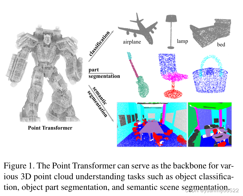
1. 研究自注意力网络在三维点云处理应用上的效果怎么样
2. 为点云设计了自注意力层，并构造了自注意力网络
3. 可以用于语义场景分割、目标部分检测和目标分类
4. 代码详见https://github.com/POSTECH-CVLab/point-transformer

1. 引言

1. Transformer很适合处理点云，因为自注意力操作具有排列和基数（cardinality）不变的特性。
2. 研究了自注意力在局部邻域和位置信息上的应用，最终的网络只基于自注意力和点的操作
3. 贡献：Point Transformer layer+Point Transformer networks+SOTA performance

2. 相关工作

Projection-based networks

1. this approach heavily relies on tangent estimation
2. the geometric information inside point clouds is collapsed during the projection stage
3. these approaches may also underutilize the sparsity of point clouds when forming dense pixel grids on projection planes
4. The choice of projection planes may heavily influence recognition performance and occlusion in 3D may impede accuracy

Voxel-based networks

1. this strategy can incur massive computation and memory costs due to
   the cubic growth in the number of voxels
2. may lose geometric detail due to quantization onto the voxel grid

Point-based networks

1. Point
2. Graph
3. Continuous convolutions

Transformer and self-attention

自注意力那么吸引我们兴趣的原因在于位置信息是通过被处理为集合的元素特性提供的， 三维点云本身就是带有位置信息的集合。

尽管之前已经有很多工作将注意力应用到点云上，但是他们都是将全局注意力用在整个点云上，计算量很大，对于大规模的点云场景理解不适用。此外，他们还用了scalar dot-product attention，不同的通道享有相同的聚合权值。

本文使用了局部自注意力机制 ，vector attention 和 合适的位置编码

3. Point Transformer

3.1 Background

令 X = { x i } i \mathcal{X}=\left\{\mathbf{x}_{i}\right\}_{i} X={xi​}i​表示一组特征向量，标准的scalar dot-product attention层可以表示为：
$${\mathbf{y}}_i=\sum _{{\mathbf{x}}_j\in \mathcal{X}}\rho \left(\phi {\left({\mathbf{x}}_i\right)}^{\top }\psi \left({\mathbf{x}}_j\right)+\delta \right)\alpha \left({\mathbf{x}}_j\right)$$
其中${\mathbf{y}}_i$ 是输出特征，$\phi ,\psi$, 和 $\alpha$是pointwise特征变换，$\delta$ 是位置编码函数， $\rho$ 是归一化函数。Scalar attention层计算了通过$\phi$ 和 $\psi$变换后特征间的scalar product，还使用输出作为注意力权值，用于聚合由$\alpha$变换后的特征。

在vector attention中，注意力权值的计算不一样，特别地，注意力权值是可以调制各自特征通道的向量：
$${\mathbf{y}}_i=\sum _{{\mathbf{x}}_j\in \mathcal{X}}\rho \left(\gamma \left(\beta \left(\phi \left({\mathbf{x}}_i\right),\psi \left({\mathbf{x}}_j\right)\right)+\delta \right)\right)\odot \alpha \left({\mathbf{x}}_j\right),$$
其中$\beta$是关联函数，$\gamma$是映射函数，用于生成特征聚合的向量。

3.2 Point Transformer Layer

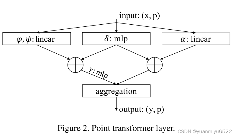
Point transformer中是基于vector的self-attention，使用了subtraction relation， 在 $\gamma$和$\alpha$中都加上了位置编码$\delta$：
$${\mathbf{y}}_i=\sum _{{\mathbf{x}}_j\in \mathcal{X}(i)}\rho \left(\gamma \left(\phi \left({\mathbf{x}}_i\right)-\psi \left({\mathbf{x}}_j\right)+\delta \right)\right)\odot \left(\alpha \left({\mathbf{x}}_j\right)+\delta \right)$$

这里，子集$\mathcal{X}(i)\subseteq \mathcal{X}$是一组${\mathbf{x}}_i$的局部相邻点，因此就可以得到局部自注意力特征。映射函数$\gamma$是一个带有两层linear和一层ReLU的MLP。

3.3 Position Encoding

在三维点云处理中，由于三维点云坐标本身就可以为位置编码提供信息，所以使用可训练的参数位置编码方法：
$$\delta =\theta \left({\mathbf{p}}_i-{\mathbf{p}}_j\right)$$
这里，${\mathbf{p}}_i$和${\mathbf{p}}_j$是点$i$和点$j$的坐标。编码函数 $\theta$是MLP。特别注意的是，我们发现，位置编码对于注意力生成分支和特征变换分支都很重要，所以在这两个地方都加了位置编码。位置编码$\theta$是通过子网络端到端训练的。

3.4 Point Transformer Block

构造了一个residual point transformer block，其中point transformer layer是核心。

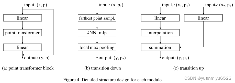
Transformer块包含了以下几个部分：

1. 自注意力层
2. bottleneck层
3. residual connection

输入是一组特征向量$\mathbf{x}$和三维坐标$\mathbf{p}$。

Point transformer block更有利于相邻特征矩阵的信息交换，从而生成新的特征向量作为输入。

3.5 Network Architecture

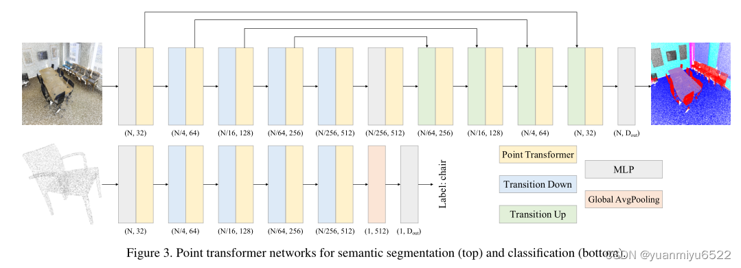
基于Point transformer block构造了一个完整的三维点云理解网络，主要的结构包括：

1. point transformer layers
2. pointwise transformations
3. pooling

3.5.1 Backbone structure

Point transformer networks中的特征编码器有五步，每一步下采样率为[1, 4, 4, 4, 4]，因此每一步的点云基数为[N, N/4, N/16, N/64, N/256]，其中N是点云的总数。

3.5.2 Transition down

Transition down用于特征编码，假设输入是${\mathcal{P}}_1$，输出是${\mathcal{P}}_2$

1. 首先执行Farthest Point Sampling (FPS)，从${\mathcal{P}}_1$中采样出${\mathcal{P}}_2$
2. 对于${\mathcal{P}}_2$中的每个点，在${\mathcal{P}}_1$中找k=16的邻域
3. 用MLP（Linear+BN+ReLU）分别对每个${\mathcal{P}}_2$对应的特征进行处理，最后再用最大池化操作得到最后的${\mathcal{P}}_2$个特征

3.5.3 Transition up

Transition up用于特征解码。
对于语义分割这些任务，利用U-Net设计，编码器和解码器对称的结构，输入是${\mathcal{P}}_2$，输出是${\mathcal{P}}_1$：

1. 输入数据先经过一个MLP（Linear+BN+ReLU）
2. 通过三线性插值恢复到${\mathcal{P}}_1$的维度
3. 与编码器中相同维度的特征进行skip connection

3.5.4 Output head

对于语义分割任务，在解码器后面加一个MLP得到最后的logits。

对于分类任务，对特征间进行全局平均池化得到全部点集的全局特征向量，在后面加一个MLP得到最后的logits。

4. 实验

1. 3D semantic segmentation ——> Stanford Large-Scale 3D Indoor Spaces (S3DIS) dataset
2. 3D shape classification ——> ModelNet40 dataset
3. 3D object part segmentation ——> ShapeNetPart

PyTorch
Momentum = 0.9
Weight decay = 0.0001

Semantic segmentation
Iterations = 40K
Initial learning rate = 0.5， dropped by 10x at steps 24K and 32K

3D shape classification & 3D object part segmentation

Epochs = 200
Initial learning rate = 0.05，dropped by 10x at epochs 120 and 160

4.1 Semantic Segmentation

S3DIS数据集包含了三个不同建筑物，六个区域，271个房间的语义信息。其中，每个点都被分配了13个类别。

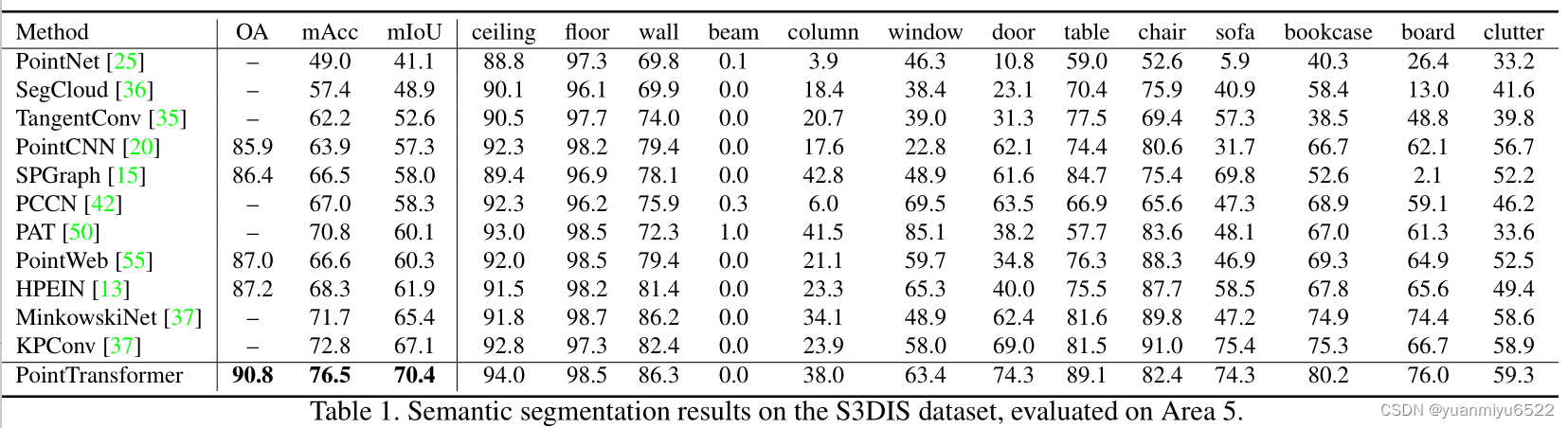
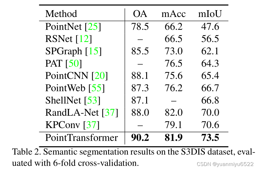
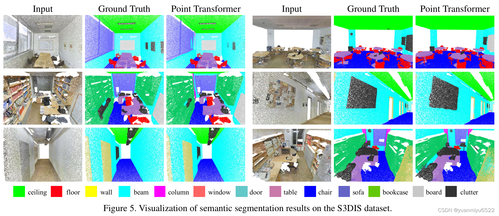
4.2 Shape Classification

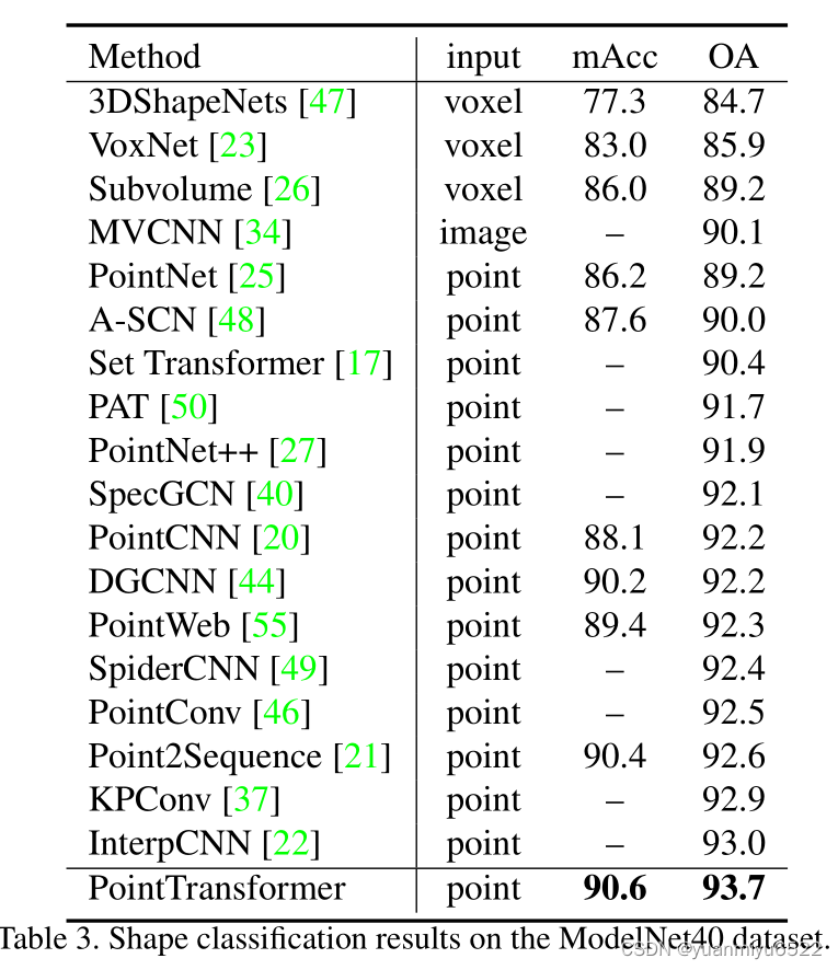
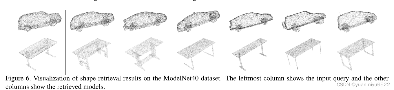
4.3 Object Part Segmentation

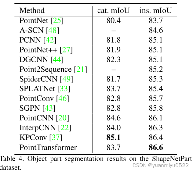
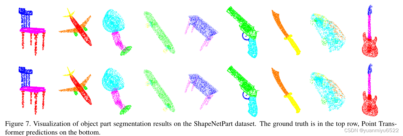
4.3 Ablation Study

消融实验主要针对S3DIS数据集在语义分割任务上的性能。

邻域的数量

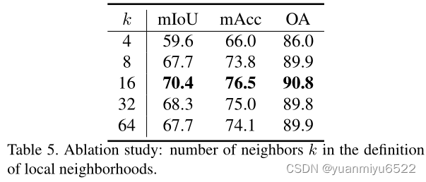
1. 如何邻域的数量太小，那么模型可能会获取不到预测的内容
2. 如果邻域的数量太大，相邻点就会太远和不相关，这可能会导致额外的噪声

Softmax 正则项 $\rho$

Point transformer w/o Softmax regularization 66.5%/72.8%/89.3%
Point transformer w Softmax regularization (70.4%/76.5%90.8%)

Position encoding $\delta$

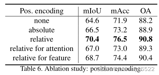
加两个位置编码很管用。

Attention type

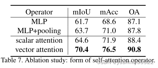
5. 结论

Transformer 可能是最适合点云处理的方法，因为点云本质上就是在度量空间上的点集嵌入，而自注意力机就是一个点集处理器。

生词

1. cardinality n. 基数
2. flesh out v. 充实