
【无人机控制】基于强化学习在无人机中调整PID参数附Matlab代码
✅作者简介:热爱科研的Matlab仿真开发者,擅长毕业设计辅导、数学建模、数据处理、程序设计科研仿真。
🍎完整代码获取 定制创新 论文复现点击:Matlab科研工作室
👇 关注我领取海量matlab电子书和数学建模资料
🍊个人信条:做科研,博学之、审问之、慎思之、明辨之、笃行之,是为:博学慎思,明辨笃行。
🔥 内容介绍
一、引言
无人机的稳定飞行依赖于精确的控制,比例 - 积分 - 微分(PID)控制器因其结构简单、鲁棒性强等优点,广泛应用于无人机的姿态和位置控制。然而,传统的 PID 参数整定方法往往依赖经验或试错,难以在复杂多变的飞行环境中实现最优控制。强化学习作为一种强大的机器学习技术,能够通过智能体与环境的交互学习,自动优化控制策略。将强化学习应用于无人机 PID 参数的调整,有望实现无人机在不同飞行条件下的自适应、最优控制。
二、PID 控制器基础
PID 控制原理
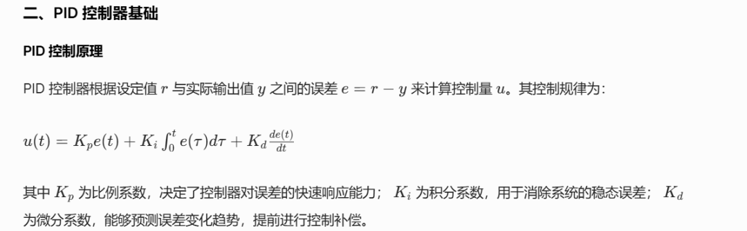
在无人机控制中,例如姿态控制,设定值可能是期望的飞行姿态角度,实际输出值为当前测量的姿态角度,通过 PID 控制器计算出的控制量用于调整无人机的电机转速或舵机角度,从而使无人机达到并保持期望的姿态。
PID 参数调整的挑战
- 环境复杂性
:无人机飞行环境复杂多变,如不同的天气条件(风速、风向变化)、飞行高度和任务要求等,这些因素都会影响无人机的动力学特性,使得固定的 PID 参数难以在各种情况下都保证良好的控制性能。
- 模型不确定性
:无人机的精确动力学模型难以建立,存在诸多不确定性因素,如机身结构的微小差异、电机性能的不一致性等。这导致基于模型的传统参数整定方法效果不佳。
三、强化学习基础
强化学习概念
强化学习是一种机器学习范式,其中智能体通过与环境进行交互,采取行动并从环境中获得奖励反馈,以学习到最优的行为策略。智能体的目标是最大化长期累积奖励。
在强化学习框架中,主要包含以下几个要素:
- 状态(State)
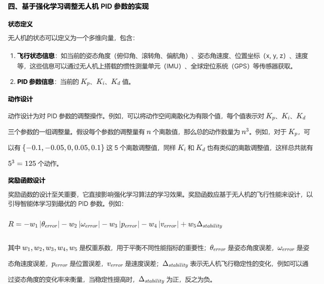
:描述智能体当前所处的环境状况。在无人机 PID 参数调整问题中,状态可以包括无人机的姿态、速度、位置等信息,以及当前的 PID 参数值。
- 动作(Action)
:智能体在某个状态下可以采取的操作。对于无人机 PID 参数调整,动作可以是对 Kp、Ki、Kd 这三个参数的调整量,例如增加或减小一定比例的参数值。
- 奖励(Reward)
:环境根据智能体的动作给予的反馈信号。在无人机控制场景中,奖励可以基于无人机的飞行性能指标来设计,如姿态误差、位置误差的减小,飞行稳定性的提高等。例如,当无人机的实际姿态更接近设定姿态时,给予正奖励;反之,若姿态误差增大,则给予负奖励。
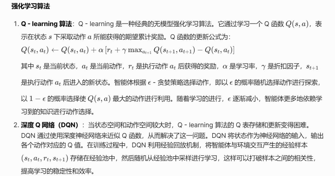
强化学习算法
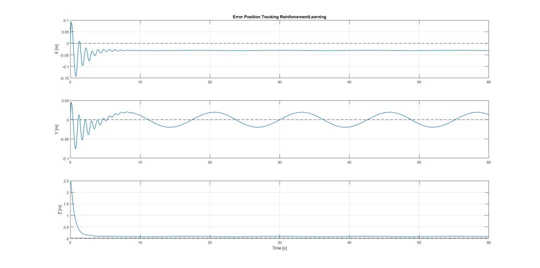
⛳️ 运行结果
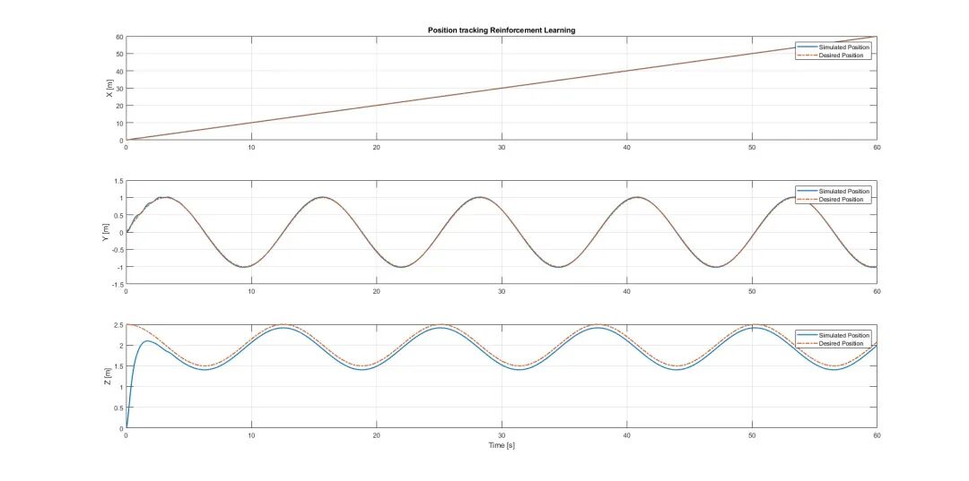
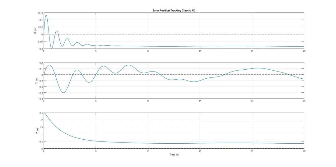
📣 部分代码
%%
% Define the desired position trajectory (3xN matrix)
% Each row corresponds to X, Y, Z components respectively.
pos_d = [RL_tout'; sin(0.5*RL_tout)'; 2 + 0.5*cos(0.5*RL_tout)'];
% Transpose pos_d to have Nx3 format — each column corresponds to one axis (X, Y, Z)
pos_d = pos_d';
% Define the desired velocity trajectory (3xN matrix)
vel_d = [ ones(size(RL_tout))'; ...
0.5*cos(0.5*RL_tout)'; ...
-0.25*sin(0.5*RL_tout)' ];
vel_d = vel_d';
%% Plot position tracking performance
figure(6)
for i=1:3
subplot(3,1,i)
% Plot simulated and desired positions over time
plot(RL_tout, RL_Tuning_Position(:,i), 'LineWidth', 1.5)
hold on
plot(RL_tout, pos_d(:,i), '-.', 'LineWidth', 1.5)
hold off
grid on
% Label each subplot according to axis
if i == 1
ylabel('X [m]')
title('Position tracking Reinforcement Learning')
elseif i == 2
ylabel('Y [m]')
else
ylabel('Z [m]')
xlabel('Time [s]')
end
% Add legend
legend('Simulated Position','Desired Position')
end
%% Plot velocity tracking performance
figure(7)
for i=1:3
subplot(3,1,i)
% Plot simulated and desired velocities
plot(RL_tout, RL_Tuning_Velocity(:,i), 'LineWidth', 1.2)
hold on
plot(RL_tout, vel_d(:,i), '-.', 'LineWidth', 1.2)
hold off
grid on
% Label each subplot according to axis
if i == 1
ylabel('X [m/s]')
title('Velocity tracking Reinforcement Learning')
elseif i == 2
ylabel('Y [m/s]')
else
ylabel('Z [m/s]')
xlabel('Time [s]')
end
% Add legend
legend('Simulated Velocity','Desired Velocity')
end
%% Plot position tracking error
figure(8)
for i=1:3
subplot(3,1,i)
% Plot position error (desired - simulated)
plot(RL_tout, pos_d(:,i)-RL_Tuning_Position(:,i), 'LineWidth', 1.2)
hold on
yline(0,'k--','LineWidth',1.2); % Reference zero line
hold off
grid on
% Label subplots
if i == 1
ylabel('X [m]')
title('Error Position Tracking Reinforcement Learning')
elseif i == 2
ylabel('Y [m]')
else
ylabel('Z [m]')
xlabel('Time [s]')
end
end
%% Plot velocity tracking error
figure(9)
for i=1:3
subplot(3,1,i)
% Plot velocity error (desired - simulated)
plot(RL_tout, vel_d(:,i)-RL_Tuning_Velocity(:,i), 'LineWidth', 1.2)
hold on
yline(0,'k--','LineWidth',1.2); % Reference zero line
hold off
grid on
% Label subplots
if i == 1
ylabel('X [m/s]')
title('Error Velocity Tracking Reinforcement Learning')
elseif i == 2
ylabel('Y [m/s]')
else
ylabel('Z [m/s]')
xlabel('Time [s]')
end
end
%% Plot angular error (orientation tracking)
Error_Ang = squeeze(RL_Tuning_Error_Ang)'; % Convert angular error data to 2D (Nx3)
figure(10)
% Plot angular errors for each axis
plot(RL_tout, Error_Ang(:,1), 'LineWidth', 1.2)
hold on
plot(RL_tout, Error_Ang(:,2), 'LineWidth', 1.2)
plot(RL_tout, Error_Ang(:,3), 'LineWidth', 1.2)
hold off
grid on
xlabel('Time [s]')
ylabel('Angular error [rad]')
title('Angular Error Classic PD')
legend('Error X','Error Y','Error Z')
%% Plot proportional gain evolution (K_P)
A = RL_Tuning_Gains.Data; % Extract gain values
T = RL_Tuning_Gains.Time; % Extract time vector
% Odd indices correspond to proportional gains (K_P)
odd_indices = 1:2:6; % 1, 3, 5
figure;
for k = 1:length(odd_indices)
i = odd_indices(k);
subplot(length(odd_indices),1,k)
plot(T, A(:,i), 'LineWidth', 1.2)
grid on;
% Label each subplot for K_P gains
switch i
case 1
ylabel('K_P X')
title('Evolution of the PD’s gains')
case 3
ylabel('K_P Y')
case 5
ylabel('K_P Z')
xlabel('Time [s]')
end
end
%% Plot derivative gain evolution (K_D)
A = RL_Tuning_Gains.Data;
T = RL_Tuning_Gains.Time;
% Even indices correspond to derivative gains (K_D)
even_indices = 2:2:6; % 2, 4, 6
figure;
for k = 1:length(even_indices)
i = even_indices(k);
subplot(length(even_indices),1,k)
plot(T, A(:,i), 'LineWidth', 1.2)
grid on;
% Label each subplot for K_D gains
switch i
case 2
ylabel('K_D X')
title('Evolution of the PD’s gains')
case 4
ylabel('K_D Y')
case 6
ylabel('K_D Z')
xlabel('Time [s]')
end
end
%% Plot all PD gains together
A = RL_Tuning_Gains.Data;
T = RL_Tuning_Gains.Time;
figure;
% Plot all six PD gains (K_P and K_D for each axis)
plot(T, A(:,1), 'LineWidth', 1.2)
hold on
plot(T, A(:,2), 'LineWidth', 1.2)
plot(T, A(:,3), 'LineWidth', 1.2)
plot(T, A(:,4), 'LineWidth', 1.2)
plot(T, A(:,5), 'LineWidth', 1.2)
plot(T, A(:,6), 'LineWidth', 1.2)
ylabel('Proportional & Derivative Gains')
xlabel('Time [s]')
legend('K_{P,new X}','K_{D,new X}','K_{P,new Y}','K_{D,new Y}','K_{P,new Z}','K_{D,new Z}')
🔗 参考文献
🍅更多免费数学建模和仿真教程关注领取
更多推荐
 0
0 0
0- 0


 已为社区贡献5条内容

所有评论(0)